In the first post of the Understanding Bayes series I said:
The likelihood is the workhorse of Bayesian inference. In order to understand Bayesian parameter estimation you need to understand the likelihood. In order to understand Bayesian model comparison (Bayes factors) you need to understand the likelihood and likelihood ratios.
I’ve shown in another post how the likelihood works as the updating factor for turning priors into posteriors for parameter estimation. In this post I’ll explain how using Bayes factors for model comparison can be conceptualized as a simple extension of likelihood ratios.
There’s that coin again
Imagine we’re in a similar situation as before: I’ve flipped a coin 100 times and it came up 60 heads and 40 tails. The likelihood function for binomial data in general is:
and for this particular result:
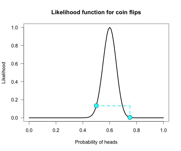
The corresponding likelihood curve is shown below, which displays the relative likelihood for all possible simple (point) hypotheses given this data. Any likelihood ratio can be calculated by simply taking the ratio of the different hypotheses’s heights on the curve.
In that previous post I compared the fair coin hypothesis — H0: P(H)=.5 — vs one particular trick coin hypothesis — H1: P(H)=.75. For 60 heads out of 100 tosses, the likelihood ratio for these hypotheses is L(.5)/L(.75) = 29.9. This means the data are 29.9 times as probable under the fair coin hypothesis than this particular trick coin hypothesis. But often we don’t have theories precise enough to make point predictions about parameters, at least not in psychology. So it’s often helpful if we can assign a range of plausible values for parameters as dictated by our theories.
Enter the Bayes factor
Calculating a Bayes factor is a simple extension of this process. A Bayes factor is a weighted average likelihood ratio, where the weights are based on the prior distribution specified for the hypotheses. For this example I’ll keep the simple fair coin hypothesis as the null hypothesis — H0: P(H)=.5 — but now the alternative hypothesis will become a composite hypothesis — H1: P(θ). (footnote 1) The likelihood ratio is evaluated at each point of P(θ) and weighted by the relative plausibility we assign that value. Then once we’ve assigned weights to each ratio we just take the average to get the Bayes factor. Figuring out how the weights should be assigned (the prior) is the tricky part.
Imagine my composite hypothesis, P(θ), is a combination of 21 different point hypotheses, all evenly spaced out between 0 and 1 and all of these points are weighted equally (not a very realistic hypothesis!). So we end up with P(θ) = {0, .05, .10, .15, . . ., .9, .95, 1}. The likelihood ratio can be evaluated at every possible point hypothesis relative to H0, and we need to decide how to assign weights. This is easy for this P(θ); we assign zero weight for every likelihood ratio that is not associated with one of the point hypotheses contained in P(θ), and we assign weights of 1 to all likelihood ratios associated with the 21 points in P(θ).
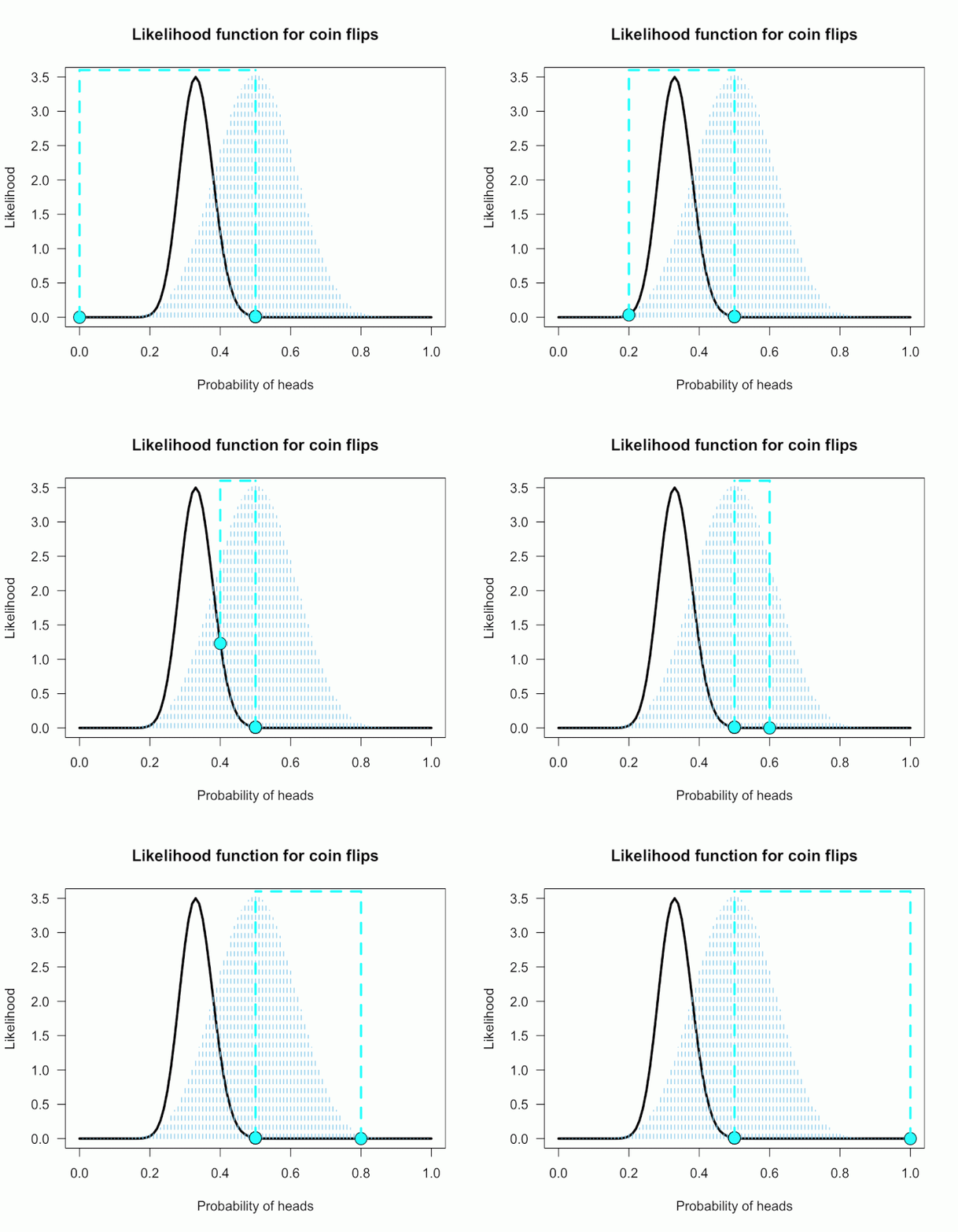
This gif has the 21 point hypotheses of P(θ) represented as blue vertical lines (indicating where we put our weights of 1), and the turquoise tracking lines represent the likelihood ratio being calculated at every possible point relative to H0: P(H)=.5. (Remember, the likelihood ratio is the ratio of the heights on the curve.) This means we only care about the ratios given by the tracking lines when the dot attached to the moving arm aligns with the vertical P(θ) lines. [edit: this paragraph added as clarification]
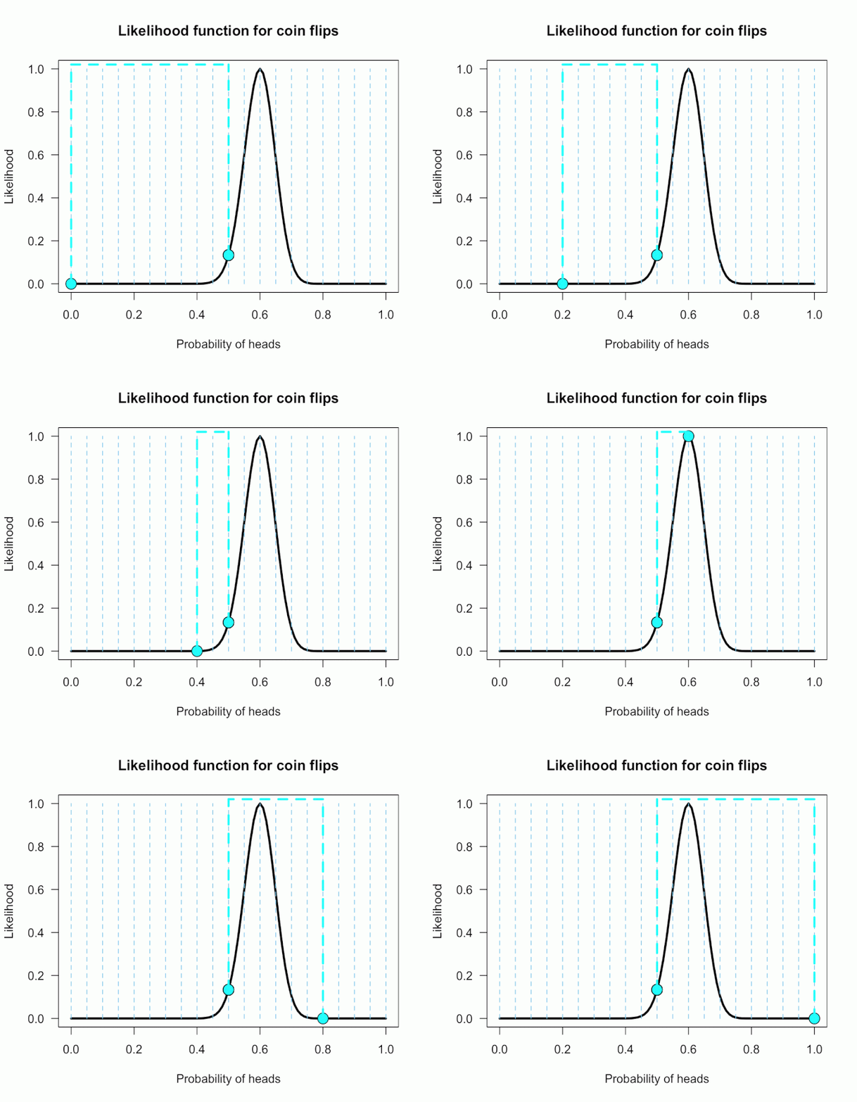
The 21 likelihood ratios associated with P(θ) are:
{~0, ~0, ~0, ~0, ~0, ~0, ~0, ~0, .002, .08, 1, 4.5, 7.5, 4.4, .78, .03, ~0, ~0, ~0, ~0, ~0}
Since they are all weighted equally we simply average, and obtain BF = 18.3/21 = .87. In other words, the data (60 heads out of 100) are 1/.87 = 1.15 times more probable under the null hypothesis — H0: P(H)=.5 — than this particular composite hypothesis — H1: P(θ). Entirely uninformative! Despite tossing the coin 100 times we have extremely weak evidence that is hardly worth even acknowledging. This happened because much of P(θ) falls in areas of extremely low likelihood relative to H0, as evidenced by those 13 zeros above. P(θ) is flexible, since it covers the entire possible range of θ, but this flexibility comes at a price. You have to pay for all of those zeros with a lower weighted average and a smaller Bayes factor.
Now imagine I had seen a trick coin like this before, and I know it had a slight bias towards landing heads. I can use this information to make more pointed predictions. Let’s say I define P(θ) as 21 equally weighted point hypotheses again, but this time they are all equally spaced between .5 and .75, which happens to be the highest density region of the likelihood curve (how fortuitous!). Now P(θ) = {.50, .5125, .525, . . ., .7375, .75}.
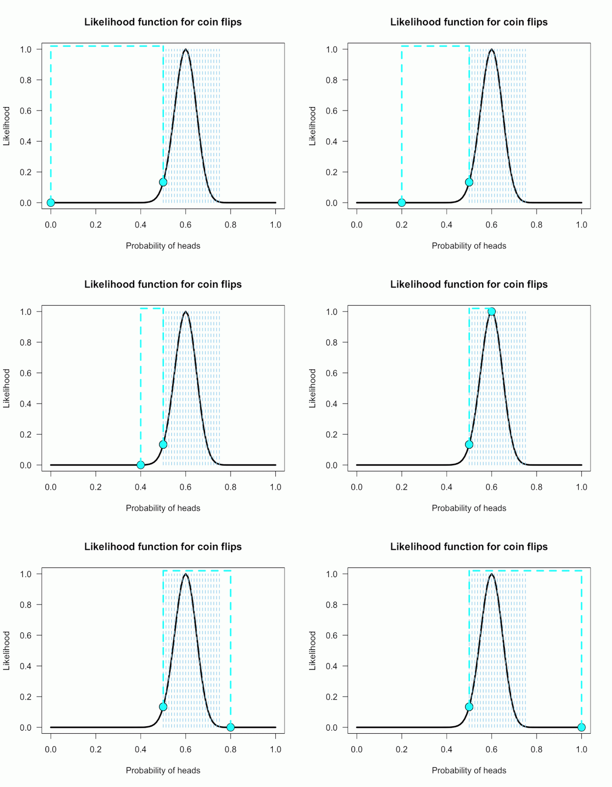
The 21 likelihood ratios associated with the new P(θ) are:
{1.00, 1.5, 2.1, 2.8, 4.5, 5.4, 6.2, 6.9, 7.5, 7.3, 6.9, 6.2, 4.4, 3.4, 2.6, 1.8, .78, .47, .27, .14, .03}
They are all still weighted equally, so the simple average is BF = 72/21 = 3.4. Three times more informative than before, and in favor of P(θ) this time! And no zeros. We were able to add theoretically relevant information to H1 to make more accurate predictions, and we get rewarded with a Bayes boost. (But this result is only 3-to-1 evidence, which is still fairly weak.)
This new P(θ) is risky though, because if the data show a bias towards tails or a more extreme bias towards heads then it faces a very heavy penalty (many more zeros). High risk = high reward with the Bayes factor. Make pointed predictions that match the data and get a bump to your BF, but if you’re wrong then pay a steep price. For example, if the data were 60 tails instead of 60 heads the BF would be 10-to-1 against P(θ) rather than 3-to-1 for P(θ)!
Now, typically people don’t actually specify hypotheses like these. Typically they use continuous distributions, but the idea is the same. Take the likelihood ratio at each point relative to H0, weigh according to plausibilities given in P(θ), and then average.
A more realistic (?) example
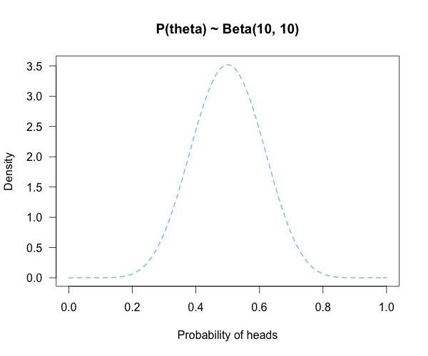
Imagine you’re walking down the sidewalk and you see a shiny piece of foreign currency by your feet. You pick it up and want to know if it’s a fair coin or an unfair coin. As a Bayesian you have to be precise about what you mean by fair and unfair. Fair is typically pretty straightforward — H0: P(H)=.5 as before — but unfair could mean anything. Since this is a completely foreign coin to you, you may want to be fairly open-minded about it. After careful deliberation, you assign P(θ) a beta distribution, with shape parameters 10 and 10. That is, H1: P(θ) ~ Beta(10, 10). This means that if the coin isn’t fair, it’s probably close to fair but it could reasonably be moderately biased, and you have no reason to think it is particularly biased to one side or the other.
Now you build a perfect coin-tosser machine and set it to toss 100 times (but not any more than that because you haven’t got all day). You carefully record the results and the coin comes up 33 heads out of 100 tosses. Under which hypothesis are these data more probable, H0 or H1? In other words, which hypothesis did the better job predicting these data?
This may be a continuous prior but the concept is exactly the same as before: weigh the various likelihood ratios based on the prior plausibility assignment and then average. The continuous distribution on P(θ) can be thought of as a set of many many point hypotheses spaced very very close together. So if the range of θ we are interested in is limited to 0 to 1, as with binomials and coin flips, then a distribution containing 101 point hypotheses spaced .01 apart, can effectively be treated as if it were continuous. The numbers will be a little off but all in all it’s usually pretty close. So imagine that instead of 21 hypotheses you have 101, and their relative plausibilities follow the shape of a Beta(10, 10). (footnote 2)
Since this is not a uniform distribution, we need to assign varying weights to each likelihood ratio. Each likelihood ratio associated with a point in P(θ) is simply multiplied by the respective density assigned to it under P(θ). For example, the density of P(θ) at .4 is 2.44. So we multiply the likelihood ratio at that point, L(.4)/L(.5) = 128, by 2.44, and add it to the accumulating total likelihood ratio. Do this for every point and then divide by the total number of points, in this case 101, to obtain the approximate Bayes factor. The total weighted likelihood ratio is 5564.9, divide it by 101 to get 55.1, and there’s the Bayes factor. In other words, the data are roughly 55 times more probable under this composite H1 than under H0. The alternative hypothesis H1 did a much better job predicting these data than did the null hypothesis H0.
The actual Bayes factor is obtained by integrating the likelihood with respect to H1’s density distribution and then dividing by the (marginal) likelihood of H0. Essentially what it does is cut P(θ) into slices infinitely thin before it calculates the likelihood ratios, re-weighs, and averages. That Bayes factor comes out to 55.7, which is basically the same thing we got through this ghetto visualization demonstration!
Take home
The take-home message is hopefully pretty clear at this point: When you are comparing a point null hypothesis with a composite hypothesis, the Bayes factor can be thought of as a weighted average of every point hypothesis’s likelihood ratio against H0, and the weights are determined by the prior density distribution of H1. Since the Bayes factor is a weighted average based on the prior distribution, it’s really important to think hard about the prior distribution you choose for H1. In a previous post, I showed how different priors can converge to the same posterior with enough data. The priors are often said to “wash out” in estimation problems like that. This is not necessarily the case for Bayes factors. The priors you choose matter, so think hard!
Notes
Footnote 1: A lot of ink has been spilled arguing about how one should define P(θ). I talked about it a little a previous post.
Footnote 2: I’ve rescaled the likelihood curve to match the scale of the prior density under H1. This doesn’t affect the values of the Bayes factor or likelihood ratios because the scaling constant cancels itself out.
R code
| ## Plots the likelihood function for the data obtained | |
| ## h = number of successes (heads), n = number of trials (flips), | |
| ## p1 = prob of success (head) on H1, p2 = prob of success (head) on H0 | |
| #the auto plot loop is taken from http://www.r-bloggers.com/automatically-save-your-plots-to-a-folder/ | |
| #and then the pngs are combined into a gif online | |
| LR <- function(h,n,p1=seq(0,1,.01),p2=rep(.5,101)){ | |
| L1 <- dbinom(h,n,p1)/dbinom(h,n,h/n) ## Likelihood for p1, standardized vs the MLE | |
| L2 <- dbinom(h,n,p2)/dbinom(h,n,h/n) ## Likelihood for p2, standardized vs the MLE | |
| Ratio <<- dbinom(h,n,p1)/dbinom(h,n,p2) ## Likelihood ratio for p1 vs p2, saves to global workspace with <<- | |
| x<- seq(0,1,.01) #sets up for loop | |
| m<- seq(0,1,.01) #sets up for p(theta) | |
| ym<-dbeta(m,10,10) #p(theta) densities | |
| names<-seq(1,length(x),1) #names for png loop | |
| for(i in 1:length(x)){ | |
| mypath<-file.path("~","Dropbox","Blog Drafts","bfs","figs1",paste("myplot_", names[i], ".png", sep = "")) #set up for save file path | |
| png(file=mypath, width=1200,height=1000,res=200) #the next plotted item saves as this png format | |
| curve(3.5*(dbinom(h,n,x)/max(dbinom(h,n,h/n))), ylim=c(0,3.5), xlim = c(0,1), ylab = "Likelihood", | |
| xlab = "Probability of heads",las=1, main = "Likelihood function for coin flips", lwd = 3) | |
| lines(m,ym, type="h", lwd=1, lty=2, col="skyblue" ) #p(theta) density | |
| points(p1[i], 3.5*L1[i], cex = 2, pch = 21, bg = "cyan") #tracking dot | |
| points(p2, 3.5*L2, cex = 2, pch = 21, bg = "cyan") #stationary null dot | |
| #abline(v = h/n, lty = 5, lwd = 1, col = "grey73") #un-hash if you want to add a line at the MLE | |
| lines(c(p1[i], p1[i]), c(3.5*L1[i], 3.6), lwd = 3, lty = 2, col = "cyan") #adds vertical line at p1 | |
| lines(c(p2[i], p2[i]), c(3.5*L2[i], 3.6), lwd = 3, lty = 2, col = "cyan") #adds vertical line at p2, fixed at null | |
| lines(c(p1[i], p2[i]), c(3.6, 3.6), lwd=3,lty=2,col="cyan") #adds horizontal line connecting them | |
| dev.off() #lets you save directly | |
| } | |
| } | |
| LR(33,100) #executes the final example | |
| v<-seq(0,1,.05) #the segments of P(theta) when it is uniform | |
| sum(Ratio[v]) #total weighted likelihood ratio | |
| mean(Ratio[v]) #average weighted likelihood ratio (i.e., BF) | |
| x<- seq(0,1,.01) #segments for p(theta)~beta | |
| y<-dbeta(x,10,10) #assigns densitys for P(theta) | |
| k=sum(y*Ratio) #multiply likelihood ratios by the density under P(theta) | |
| l=k/101 #weighted average likelihood ratio (i.e., BF) | |
[…] Understanding Bayes: Visualization of the Bayes Factor […]
Hi Alex,
once again, an excellent blog post! I’ve taken your binomial example and made a shiny app out of it (also does Bayes factors). Might be of use! https://gist.github.com/dostodabsi/0f176eb25e2e722ec040
cheers,
Fabian
[…] how this could be done for many types of problems. The approach naturally leads to computing a Bayes factor. With Bayes factors, one must explicitly define the hypotheses (models) being compared. In this […]
[…] how this could be done for many types of problems. The approach naturally leads to computing a Bayes factor. With Bayes factors, one must explicitly define the hypotheses (models) being compared. In […]
[…] Bayes I want to discuss the nature of Bayesian evidence and conclusions. In a previous post I focused on Bayes factors’ mathematical structure and visualization. In this post I hope to […]
[…] in the sample has to be interpreted in the context of the specific problem. I didn’t go into Bayes factors or posterior estimation because I promised that it would be a simple and easy talk about the basic […]
thanks for excellent tutoring! cos the pdf is a continuous variable,the total number of points is positive infinite.what number should be divide by?
[…] a B for every p.” Meaning, for every p value in the paper report a corresponding Bayes factor. This way the psychology community can start to build an intuition about how these two kinds of […]
[…] Understanding Bayes: Visualization of the Bayes Factor | The Etz-Files […]
I see some reporting the natural log of the Bayes Factor. Why might one want to report that instead of the Bayes Factor? How does interpretation differ?
Taking the log of the BF makes the evidence from independent sources additive rather than multiplicative, which some find more intuitive. Turing did this during WWII using what he called “decibans” to measure accumulation of the evidence when cracking the German enigma codes.
In section Enter the Bayes factor, you have the example of comparing a point hypothesis of 0.5 to the composite hypothesis of having 21 different point hypotheses between 0 and 1. Why is 0.5 part of the composite hypothesis, H1? Wouldn’t that be excluded, since it’s the H0 hypothesis? Thus, you would have 20 points instead of 21, and no longer have the likelihood ratio of 1 in the string of likelihood ratios to be summed?
[…] effects an RCT testing an effective intervention might find, and calculate a statistic known as a Bayes Factor. This quantifies which of our two hypotheses the RCT’s results are more consistent with. […]
[…] factor. As has been shown earlier, likelihood ratios and Bayes factors are closely related (see here for a visual display of the relationship). Both quantities measure the relative evidence for one […]
[…] factor. As has been shown earlier, likelihood ratios and Bayes factors are closely related (see here for a visual display of the relationship). Both quantities measure the relative evidence for one […]