I recently gave a talk at the University of Bristol’s Medical Research Council Integrative Epidemiology Unit, titled, “A Bayesian Perspective on the Reproducibility Project: Psychology,” in which I recount the results from our recently published Bayesian reanalysis of the RPP (you can read it in PLOS ONE). In that paper Joachim Vandekerckhove and I reassessed the evidence from the RPP and found that most of the original and replication studies only managed to obtain weak evidence.
I’m very grateful to Marcus Munafo for inviting me out to give this talk. And I’m also grateful to Jim Lumsden for help organizing. We recorded the talk’s audio and synced it to a screencast of my slides, so if you weren’t there you can still hear about it. 🙂
I’ve posted the slides on slideshare, and you can download a copy of the presentation by clicking here. (It says 83 slides, but the last ~30 slides are a technical appendix prepared for the Q&A)
It is sometimes considered a paradox that the answer depends not only on the observations but on the question; it should be a platitude.
–Harold Jeffreys, 1939
Joachim Vandekerckhove (@VandekerckhoveJ) and I have just published a Bayesian reanalysis of the Reproducibility Project: Psychology in PLOS ONE (CLICK HERE). It is open access, so everyone can read it! Boo paywalls! Yay open access! The review process at PLOS ONE was very nice; we had two rounds of reviews that really helped us clarify our explanations of the method and results.
Oh and it got a new title: “A Bayesian perspective on the Reproducibility Project: Psychology.” A little less presumptuous than the old blog’s title. Thanks to the RPP authors sharing all of their data, we research parasites were able to find some interesting stuff. (And thanks Richard Morey (@richarddmorey) for making this great badge)
TLDR: One of the main takeaways from the paper is the following: We shouldn’t be too surprised when psychology experiments don’t replicate, given the evidence in the original studies is often unacceptably weak to begin with!
What did we do?
Here is the abstract from the paper:
We revisit the results of the recent Reproducibility Project: Psychology by the Open Science Collaboration. We compute Bayes factors—a quantity that can be used to express comparative evidence for an hypothesis but also for the null hypothesis—for a large subset (N = 72) of the original papers and their corresponding replication attempts. In our computation, we take into account the likely scenario that publication bias had distorted the originally published results. Overall, 75% of studies gave qualitatively similar results in terms of the amount of evidence provided. However, the evidence was often weak (i.e., Bayes factor < 10). The majority of the studies (64%) did not provide strong evidence for either the null or the alternative hypothesis in either the original or the replication, and no replication attempts provided strong evidence in favor of the null. In all cases where the original paper provided strong evidence but the replication did not (15%), the sample size in the replication was smaller than the original. Where the replication provided strong evidence but the original did not (10%), the replication sample size was larger. We conclude that the apparent failure of the Reproducibility Project to replicate many target effects can be adequately explained by overestimation of effect sizes (or overestimation of evidence against the null hypothesis) due to small sample sizes and publication bias in the psychological literature. We further conclude that traditional sample sizes are insufficient and that a more widespread adoption of Bayesian methods is desirable.
In the paper we try to answer four questions: 1) How much evidence is there in the original studies? 2) If we account for the possibility of publication bias, how much evidence is left in the original studies? 3) How much evidence is there in the replication studies? 4) How consistent is the evidence between (bias-corrected) original studies and replication studies?
We implement a very neat technique called Bayesian model averaging to account for publication bias in the original studies. The method is fairly technical, so I’ve put the topic in the Understanding Bayes queue (probably the next post in the series). The short version is that each Bayes factor consists of eight likelihood functions that get weighted based on the potential bias in the original result. There are details in the paper, and much more technical detail in this paper (Guan and Vandekerckhove, 2015). Since the replication studies would be published regardless of outcome, and were almost certainly free from publication bias, we can calculate regular (bias free) Bayes factors for them.
Results
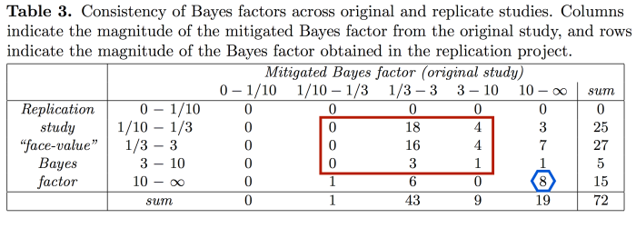
There are only 8 studies where both the bias mitigated original Bayes factors and the replication Bayes factors are above 10 (highlighted with the blue hexagon). That is, both experiment attempts provide strong evidence. It may go without saying, but I’ll say it anyway: These are the ideal cases.
(The prior distribution for all Bayes factors is a normal distribution with mean of zero and variance of one. All the code is online HERE if you’d like to see how different priors change the result; our sensitivity analysis didn’t reveal any major dependencies on the exact prior used.)
The majority of studies (46/72) have both bias mitigated original and replication Bayes factors in the 1/10< BF <10 range (highlighted with the red box). These are cases where both study attempts only yielded weak evidence.
Overall, both attempts for most studies provided only weak evidence. There is a silver/bronze/rusty-metal lining, in that when both study attempts obtain only weak Bayes factors, they are technically providing consistent amounts of evidence. But that’s still bad, because “consistency” just means that we are systematically gathering weak evidence!
Using our analysis, no studies provided strong evidence that favored the null hypothesis in either the original or replication.
It is interesting to consider the cases where one study attempt found strong evidence but another did not. I’ve highlighted these cases in blue in the table below. What can explain this?
One might be tempted to manufacture reasons that explain this pattern of results, but before you do that take a look at the figure below. We made this figure to highlight one common aspect of all study attempts that find weak evidence in one attempt and strong evidence in another: Differences in sample size. In all cases where the replication found strong evidence and the original study did not, the replication attempt had the larger sample size. Likewise, whenever the original study found strong evidence and the replication did not, the original study had a larger sample size.
Figure 2. Evidence resulting from replicated studies plotted against evidence resulting from the original publications. For the original publications, evidence for the alternative hypothesis was calculated taking into account the possibility of publication bias. Small crosses indicate cases where neither the replication nor the original gave strong evidence. Circles indicate cases where one or the other gave strong evidence, with the size of each circle proportional to the ratio of the replication sample size to the original sample size (a reference circle appears in the lower right). The area labeled ‘replication uninformative’ contains cases where the original provided strong evidence but the replication did not, and the area labeled ‘original uninformative’ contains cases where the reverse was true. Two studies that fell beyond the limits of the figure in the top right area (i.e., that yielded extremely large Bayes factors both times) and two that fell above the top left area (i.e., large Bayes factors in the replication only) are not shown. The effect that relative sample size has on Bayes factor pairs is shown by the systematic size difference of circles going from the bottom right to the top left. All values in this figure can be found in S1 Table.
Abridged conclusion (read the paper for more! More what? Nuance, of course. Bayesians are known for their nuance…)
Even when taken at face value, the original studies frequently provided only weak evidence when analyzed using Bayes factors (i.e., BF < 10), and as you’d expect this already small amount of evidence shrinks even more when you take into account the possibility of publication bias. This has a few nasty implications. As we say in the paper,
In the likely event that [the original] observed effect sizes were inflated … the sample size recommendations from prospective power analysis will have been underestimates, and thus replication studies will tend to find mostly weak evidence as well.
According to our analysis, in which a whopping 57 out of 72 replications had 1/10 < BF < 10, this appears to have been the case.
We also should be wary of claims about hidden moderators. We put it like this in the paper,
The apparent discrepancy between the original set of results and the outcome of the Reproducibility Project can be adequately explained by the combination of deleterious publication practices and weak standards of evidence, without recourse to hypothetical hidden moderators.
Of course, we are not saying that hidden moderators could not have had an influence on the results of the RPP. The statement is merely that we can explain the results reasonably well without necessarily bringing hidden moderators into the discussion. As Laplace would say: We have no need of that hypothesis.
So to sum up,
From a Bayesian reanalysis of the Reproducibility Project: Psychology, we conclude that one reason many published effects fail to replicate appears to be that the evidence for their existence was unacceptably weak in the first place.
With regard to interpretation of results — I will include the same disclaimer here that we provide in the paper:
It is important to keep in mind, however, that the Bayes factor as a measure of evidence must always be interpreted in the light of the substantive issue at hand: For extraordinary claims, we may reasonably require more evidence, while for certain situations—when data collection is very hard or the stakes are low—we may satisfy ourselves with smaller amounts of evidence. For our purposes, we will only consider Bayes factors of 10 or more as evidential—a value that would take an uninvested reader from equipoise to a 91% confidence level. Note that the Bayes factor represents the evidence from the sample; other readers can take these Bayes factors and combine them with their own personal prior odds to come to their own conclusions.
All of the results are tabulated in the supplementary materials (HERE) and the code is on github (CODE HERE).
More disclaimers, code, and differences from the old reanalysis
Disclaimer:
All of the results are tabulated in a table in the supplementary information (link), and MATLAB code to reproduce the results and figures is provided online (CODE HERE). When interpreting these results, we use a Bayes factor threshold of 10 to represent strong evidence. If you would like to see how the results change when using a different threshold, all you have to do is change the code in line 118 of the ‘bbc_main.m’ file to whatever thresholds you prefer.
#######
Important note: The function to calculate the mitigated Bayes factors is a prototype and is not robust to misuse. You should not use it unless you know what you are doing!
#######
A few differences between this paper and an old reanalysis:
A few months back I posted a Bayesian reanalysis of the Reproducibility Project: Psychology, in which I calculated replication Bayes factors for the RPP studies. This analysis took the posterior distribution from the original studies as the prior distribution in the replication studies to calculate the Bayes factor. So in that calculation, the hypotheses being compared are: H_0 “There is no effect” vs. H_A “The effect is close to that found by the original study.” It also did not take into account publication bias.
This is important: The published reanalysis is very different from the one in the first blog post.
Since the posterior distributions from the original studies were usually centered on quite large effects, the replication Bayes factors could fall in a wide range of values. If a replication found a moderately large effect, comparable to the original, then the Bayes factor would very largely favor H_A. If the replication found a small-to-zero effect (or an effect in the opposite direction), the Bayes factor would very largely favor H_0. If the replication found an effect in the middle of the two hypotheses, then the Bayes factor would be closer to 1, meaning the data fit both hypotheses equally bad. This last case happened when the replications found effects in the same direction as the original studies but of smaller magnitude.
These three types of outcomes happened with roughly equal frequency; there were lots of strong replications (big BF favoring H_A), lots of strong failures to replicate (BF favoring H_0), and lots of ambiguous results (BF around 1).
The results in this new reanalysis are not as extreme because the prior distribution for H_A is centered on zero, which means it makes more similar predictions to H_0 than the old priors. Whereas roughly 20% of the studies in the first reanalysis were strongly in favor of H_0 (BF>10), that did not happen a single time in the new reanalysis. This new analysis also includes the possibility of a biased publication processes, which can have a large effect on the results.
We use a different prior so we get different results. Hence the Jeffreys quote at the top of the page.
[Edit: There is a now-published Bayesian reanalysis of the RPP. See here.]
The Reproducibility Project was finally published this week in Science, and an outpouring ofmedia articles followed. Headlines included “More Than 50% Psychology Studies Are Questionable: Study”, “Scientists Replicated 100 Psychology Studies, and Fewer Than Half Got the Same Results”, and “More than half of psychology papers are not reproducible”.
Are these categorical conclusions warranted? If you look at the paper, it makes very clear that the results do not definitively establish effects as true or false:
After this intensive effort to reproduce a sample of published psychological findings, how many of the effects have we established are true? Zero. And how many of the effects have we established are false? Zero. Is this a limitation of the project design? No. It is the reality of doing science, even if it is not appreciated in daily practice. (p. 7)
Very well said. The point of this project was not to determine what proportion of effects are “true”. The point of this project was to see what results are replicable in an independent sample.The question arises of what exactly this means. Is an original study replicable if the replication simply matches it in statistical significance and direction? The authors entertain this possibility:
A straightforward method for evaluating replication is to test whether the replication shows a statistically significant effect (P < 0.05) with the same direction as the original study. This dichotomous vote-counting method is intuitively appealing and consistent with common heuristics used to decide whether original studies “worked.” (p. 4)
How did the replications fare? Not particularly well.
Ninety-seven of 100 (97%) effects from original studies were positive results … On the basis of only the average replication power of the 97 original, significant effects [M = 0.92, median (Mdn) = 0.95], we would expect approximately 89 positive results in the replications if all original effects were true and accurately estimated; however, there were just 35 [36.1%; 95% CI = (26.6%, 46.2%)], a significant reduction … (p. 4)
So the replications, being judged on this metric, did (frankly) horribly when compared to the original studies. Only 35 of the studies achieved significance, as opposed to the 89 expected and the 97 total. This gives a success rate of either 36% (35/97) out of all studies, or 39% (35/89) relative to the number of studies expected to achieve significance based on power calculations. Either way, pretty low. These were the numbers that most of the media latched on to.
Does this metric make sense? Arguably not, since the “difference between significant and not significant is not necessarily significant” (Gelman & Stern, 2006). Comparing significance levels across experiments is not valid inference. A non-significant replication result can be entirely consistent with the original effect, and yet count as a failure because it did not achieve significance. There must be a better metric.
The authors recognize this, so they also used a metric that utilized confidence intervals over simple significance tests. Namely, does the confidence interval from the replication study include the originally reported effect? They write,
This method addresses the weakness of the first test that a replication in the same direction and a P value of 0.06 may not be significantly different from the original result. However, the method will also indicate that a replication “fails” when the direction of the effect is the same but the replication effect size is significantly smaller than the original effect size … Also, the replication “succeeds” when the result is near zero but not estimated with sufficiently high precision to be distinguished from the original effect size. (p. 4)
So with this metric a replication is considered successful if the replication result’s confidence interval contains the original effect, and fails otherwise. The replication effect can be near zero, but if the CI is wide enough it counts as a non-failure (i.e., a “success”). A replication can also be quite near the original effect but have high precision, thus excluding the original effect and “failing”.
This metric is very indirect, and their use of scare-quotes around “succeeds” is telling. Roughly 47% of confidence intervals in the replications “succeeded” in capturing the original result. The problem with this metric is obvious: Replications with effects near zero but wide CIs get the same credit as replications that were bang on the original effect (or even larger) with narrow CIs. Results that don’t flat out contradict the original effects count as much as strong confirmations? Why should both of these types of results be considered equally successful?
Based on these two metrics, the headlines are accurate: Over half of the replications “failed”. But these two reproducibility metrics are either invalid (comparing significance levels across experiments) or very vague (confidence interval agreement). They also only offer binary answers: A replication either “succeeds” or “fails”, and this binary thinking leads to absurd conclusions in some cases like those mentioned above. Is replicability really so black and white? I will explain below how I think we should measure replicability in a Bayesian way, with a continuous measure that can find reasonable answers with replication effects near zero with wide CIs, effects near the original with tight CIs, effects near zero with tight CIs, replication effects that go in the opposite direction, and anything in between.
A Bayesian metric of reproducibility
I wanted to look at the results of the reproducibility project through a Bayesian lens. This post should really be titled, “A Bayesian …” or “One Possible Bayesian …” since there is no single Bayesian answer to any question (but those titles aren’t as catchy). It depends on how you specify the problem and what question you ask. When I look at the question of replicability, I want to know if is there evidence for replication success or for replication failure, and how strong that evidence is. That is, should I interpret the replication results as more consistent with the original reported result or more consistent with a null result, and by how much?
Verhagen and Wagenmakers (2014), and Wagenmakers, Verhagen, and Ly (2015) recently outlined how this could be done for many types of problems. The approach naturally leads to computing a Bayes factor. With Bayes factors, one must explicitly define the hypotheses (models) being compared. In this case one model corresponds to a probability distribution centered around the original finding (i.e. the posterior), and the second model corresponds to the null model (effect = 0). The Bayes factor tells you which model the replication result is more consistent with, and larger Bayes factors indicate a better relative fit. So it’s less about obtaining evidence for the effect in general and more about gauging the relative predictive success of the original effects. (footnote 1)
If the original results do a good job of predicting replication results, the original effect model will achieve a relatively large Bayes factor. If the replication results are much smaller or in the wrong direction, the null model will achieve a large Bayes factor. If the result is ambiguous, there will be a Bayes factor near 1. Again, the question is which model better predicts the replication result? You don’t want a null model to predict replication results better than your original reported effect.
A key advantage of the Bayes factor approach is that it allows natural grades of evidence for replication success. A replication result can strongly agree with the original effect model, it can strongly agree with a null model, or it can lie somewhere in between. To me, the biggest advantage of the Bayes factor is it disentangles the two types of results that traditional significance tests struggle with: a result that actually favors the null model vs a result that is simply insensitive. Since the Bayes factor is inherently a comparative metric, it is possible to obtain evidence for the null model over the tested alternative. This addresses my problem I had with the above metrics: Replication results bang on the original effects get big boosts in the Bayes factor, replication results strongly inconsistent with the original effects get big penalties in the Bayes factor, and ambiguous replication results end up with a vague Bayes factor.
Bayes factor methods are often criticized for being subjective, sensitive to the prior, and for being somewhat arbitrary. Specifying the models is typically hard, and sometimes more arbitrary models are chosen for convenience for a given study. Models can also be specified by theoretical considerations that often appear subjective (because they are). For a replication study, the models are hardly arbitrary at all. The null model corresponds to that of a skeptic of the original results, and the alternative model corresponds to a strong theoretical proponent. The models are theoretically motivated and answer exactly what I want to know: Does the replication result fit more with the original effect model or a null model? Or as Verhagen and Wagenmakers (2014) put it, “Is the effect similar to what was found before, or is it absent?” (p.1458 here).
Replication Bayes factors
In the following, I take the effects reported in figure 3 of the reproducibility project (the pretty red and green scatterplot) and calculate replication Bayes factors for each one. Since they have been converted to correlation measures, replication Bayes factors can easily be calculated using the code provided by Wagenmakers, Verhagen, and Ly (2015). The authors of the reproducibility project kindly provide the script for making their figure 3, so all I did was take the part of the script that compiled the converted 95 correlation effect sizes for original and replication studies. (footnote 2) The replication Bayes factor script takes the correlation coefficients from the original studies as input, calculates the corresponding original effect’s posterior distribution, and then compares the fit of this distribution and the null model to the result of the replication. Bayes factors larger than 1 indicate the original effect model is a better fit, Bayes factors smaller than 1 indicate the null model is a better fit. Large (or really small) Bayes factors indicate strong evidence, and Bayes factors near 1 indicate a largely insensitive result.
The replication Bayes factors are summarized in the figure below (click to enlarge). The y-axis is the count of Bayes factors per bin, and the different bins correspond to various strengths of replication success or failure. Results that fall in the bins left of center constitute support the null over the original result, and vice versa. The outer-most bins on the left or right contain the strongest replication failures and successes, respectively. The bins labelled “Moderate” contain the more muted replication successes or failures. The two central-most bins labelled “Insensitive” contain results that are essentially uninformative.
So how did we do?
You’ll notice from this crude binning system that there is quite a spread from super strong replication failure to super strong replication success. I’ve committed the sin of binning a continuous outcome, but I think it serves as a nice summary. It’s important to remember that Bayes factors of 2.5 vs 3.5, while in different bins, aren’t categorically different. Bayes factors of 9 vs 11, while in different bins, aren’t categorically different. Bayes factors of 15 and 90, while in the same bin, are quite different. There is no black and white here. These are the categories Bayesians often use to describe grades of Bayes factors, so I use them since they are familiar to many readers. If you have a better idea for displaying this please leave a comment. 🙂 Check out the “Results” section at the end of this post to see a table which shows the study number, the N in original and replications, the r values of each study, the replication Bayes factor and category I gave it, and the replication p-value for comparison with the Bayes factor. This table shows the really wide spread of the results. There is also code in the “Code” section to reproduce the analyses.
Strong replication failures and strong successes
Roughly 20% (17 out of 95) of replications resulted in relatively strong replication failures (2 left-most bins), with resultant Bayes factors at least 10:1 in favor of the null. The highest Bayes factor in this category was over 300,000 (study 110, “Perceptual mechanisms that characterize gender differences in decoding women’s sexual intent”). If you were skeptical of these original effects, you’d feel validated in your skepticism after the replications. If you were a proponent of the original effects’ replicability you’ll perhaps want to think twice before writing that next grant based around these studies.
Roughly 25% (23 out of 95) of replications resulted in relatively strong replication successes (2 right-most bins), with resultant Bayes factors at least 10:1 in favor of the original effect. The highest Bayes factor in this category was 1.3×10^32 (or log(bf)=74; study 113, “Prescribed optimism: Is it right to be wrong about the future?”) If you were a skeptic of the original effects you should update your opinion to reflect the fact that these findings convincingly replicated. If you were a proponent of these effects you feel validation in that they appear to be robust.
These two types of results are the most clear-cut: either the null is strongly favored or the original reported effect is strongly favored. Anyone who was indifferent to these effects has their opinion swayed to one side, and proponents/skeptics are left feeling either validated or starting to re-evaluate their position. There was only 1 very strong (BF>100) failure to replicate but there were quite a few very strong replication successes (16!). There were approximately twice as many strong (10<BF<100) failures to replicate (16) than strong replication successes (7).
Moderate replication failures and moderate successes
The middle-inner bins are labelled “Moderate”, and contain replication results that aren’t entirely convincing but are still relatively informative (3<BF<10). The Bayes factors in the upper end of this range are somewhat more convincing than the Bayes factors in the lower end of this range.
Roughly 20% (19 out of 95) of replications resulted in moderate failures to replicate (third bin from the left), with resultant Bayes factors between 10:1 and 3:1 in favor of the null. If you were a proponent of these effects you’d feel a little more hesitant, but you likely wouldn’t reconsider your research program over these results. If you were a skeptic of the original effects you’d feel justified in continued skepticism.
Roughly 10% (9 out of 95) of replications resulted in moderate replication successes (third bin from the right), with resultant Bayes factors between 10:1 and 3:1 in favor of the original effect. If you were a big skeptic of the original effects, these replication results likely wouldn’t completely change your mind (perhaps you’d be a tad more open minded). If you were a proponent, you’d feel a bit more confident.
Many uninformative “failed” replications
The two central bins contain replication results that are insensitive. In general, Bayes factors smaller than 3:1 should be interpreted only as very weak evidence. That is, these results are so weak that they wouldn’t even be convincing to an ideal impartial observer (neither proponent nor skeptic). These two bins contain 27 replication results. Approximately 30% of the replication results from the reproducibility project aren’t worth much inferentially!
A few examples:
Study 2, “Now you see it, now you don’t: repetition blindness for nonwords” BF = 2:1 in favor of null
Study 12, “When does between-sequence phonological similarity promote irrelevant sound disruption?” BF = 1.1:1 in favor of null
Study 80, “The effects of an implemental mind-set on attitude strength.” BF = 1.2:1 in favor of original effect
Study 143, “Creating social connection through inferential reproduction: Loneliness and perceived agency in gadgets, gods, and greyhounds” BF = 2:1 in favor of null
I just picked these out randomly. The types of replication studies in this inconclusive set range from attentional blink (study 2), to brain mapping studies (study 55), to space perception (study 167), to cross national comparisons of personality (study 154).
Should these replications count as “failures” to the same extent as the ones in the left 2 bins? Should studies with a Bayes factor of 2:1 in favor of the original effect count as “failures” as much as studies with 50:1 against? I would argue they should not, they should be called what they are: entirely inconclusive.
Interestingly, study 143 mentioned above was recently called out in this NYT article as a high-profile study that “didn’t hold up”. Actually, we don’t know if it held up! Identifying replications that were inconclusive using this continuous range helps avoid over-interpreting ambiguous results as “failures”.
Wrap up
To summarize the graphic and the results discussed above, this method identifies roughly as many replications with moderate success or better (BF>3) as the counting significance method (32 vs 35). (footnote 3) These successes can be graded based on their replication Bayes factor as moderate to very strong. The key insight from using this method is that many replications that “fail” based on the significance count are actually just inconclusive. It’s one thing to give equal credit to two replication successes that are quite different in strength, but it’s another to call all replications failures equally bad when they show a highly variable range. Calling a replication a failure when it is actually inconclusive has consequences for the original researcher and the perception of the field.
As opposed to the confidence interval metric, a replication effect centered near zero with a wide CI will not count as a replication success with this method; it would likely be either inconclusive or weak evidence in favor of the null. Some replications are indeed moderate to strong failures to replicate (36 or so), but nearly 30% of all replications in the reproducibility project (27 out of 95) were not very informative in choosing between the original effect model and the null model.
So to answer my question as I first posed it, are the categorical conclusions of wide-scale failures to replicate by the media stories warranted? As always, it depends.
If you count “success” as any Bayes factor that has any evidence in favor of the original effect (BF>1), then there is a 44% success rate (42 out of 95).
If you count “success” as any Bayes factor with at least moderate evidence in favor of the original effect (BF>3), then there is a 34% success rate (32 out of 95).
If you count “failure” as any Bayes factor that has at least moderate evidence in favor of the null (BF<1/3), then there is a 38% failure rate (36 out of 95).
If you only consider the effects sensitive enough to discriminate the null model and the original effect model (BF>3 or BF<1/3) in your total, then there is a roughly 47% success rate (32 out of 68). This number jives (uncannily) well with the prediction John Ioannidis made 10 years ago (47%).
However you judge it, the results aren’t exactly great.
But if we move away from dichotomous judgements of replication success/failure, we see a slightly less grim picture. Many studies strongly replicated, many studies strongly failed, but many studies were in between. There is a wide range! Judgements of replicability needn’t be black and white. And with more data the inconclusive results could have gone either way. I would argue that any study with 1/3<BF<3 shouldn’t count as a failure or a success, since the evidence simply is not convincing; I think we should hold off judging these inconclusive effects until there is stronger evidence. Saying “we didn’t learn much about this or that effect” is a totally reasonable thing to do. Boo dichotomization!
Try out this method!
All in all, I think the Bayesian approach to evaluating replication success is advantageous in 3 big ways: It avoids dichotomizing replication outcomes, it gives an indication of the range of the strength of replication successes or failures, and it identifies which studies we need to give more attention to (insensitive BFs). The Bayes factor approach used here can straighten out when a replication shows strong evidence in favor of the null model, strong evidence in favor of the original effect model, or evidence that isn’t convincingly in favor of either position. Inconclusive replications should be targeted for future replication, and perhaps we should look into why these studies that purport to have high power (>90%) end up with insensitive results (large variance, design flaw, overly optimistic power calcs, etc). It turns out that having high power in planning a study is no guarantee that one actually obtains convincingly sensitive data (Dienes, 2014; Wagenmakers et al., 2014).
I should note, the reproducibility project did try to move away from the dichotomous thinking about replicability by correlating the converted effect sizes (r) between original and replication studies. This was a clever idea, and it led to a very pretty graph (figure 3) and some interesting conclusions. That idea is similar in spirit to what I’ve laid out above, but its conclusions can only be drawn from batches of replication results. Replication Bayes factors allow one to compare the original and replication results on an effect by effect basis. This Bayesian method can grade a replication on its relative success or failure even if your reproducibility project only has 1 effect in it.
I should also note, this analysis is inherently context dependent. A different group of studies could very well show a different distribution of replication Bayes factors, where each individual study has a different prior distribution (based on the original effect). I don’t know how much these results would generalize to other journals or other fields, but I would be interested to see these replication Bayes factors employed if systematic replication efforts ever do catch on in other fields.
Acknowledgements and thanks
The authors of the reproducibility project have done us all a great service and I am grateful that they have shared all of their code, data, and scripts. This re-analysis wouldn’t have been possible without their commitment to open science. I am also grateful to EJ Wagenmakers, Josine Verhagen, and Alexander Ly for sharing the code to calculate the replication Bayes factors on the OSF. Many thanks to Chris Engelhardt and Daniel Lakens for some fruitful discussions when I was planning this post. Of course, the usual disclaimer applies and all errors you find should be attributed only to me.
Notes
footnote 1: Of course, a model that takes publication bias into account could fit better by tempering the original estimate, and thus show relative evidence for the bias-corrected effect vs either of the other models; but that’d be answering a different question than the one I want to ask.
footnote 2: I left out 2 results that I couldn’t get to work with the calculations. Studies 46 and 139, both appear to be fairly strong successes, but I’ve left them out of the reported numbers because I couldn’t calculate a BF.
footnote 3: The cutoff of BF>3 isn’t a hard and fast rule at all. Recall that this is a continuous measure. Bayes factors are typically a little more conservative than significance tests in supporting the alternative hypothesis. If the threshold for success is dropped to BF>2 the number of successes is 35 — an even match with the original estimate.
Results
This table is organized from smallest replication Bayes factor to largest (i.e., strongest evidence in favor of null to strongest evidence in favor of original effect). The Ns were taken from the final columns in the master data sheet,”T_N_O_for_tables” and “T_N_R_for_tables”. Some Ns are not integers because they presumably underwent df correction. There is also the replication p-value for comparison; notice that BFs>3 generally correspond to ps less than .05 — BUT there are some cases where they do not agree. If you’d like to see more about the studies you can check out the master data file in the reproducibility project OSF page (linked below).
This file contains hidden or bidirectional Unicode text that may be interpreted or compiled differently than what appears below. To review, open the file in an editor that reveals hidden Unicode characters.
Learn more about bidirectional Unicode characters
If you want to check/modify/correct my code, here it is. If you find a glaring error please leave a comment below or tweet at me 🙂
This file contains hidden or bidirectional Unicode text that may be interpreted or compiled differently than what appears below. To review, open the file in an editor that reveals hidden Unicode characters.
Learn more about bidirectional Unicode characters
Dienes, Z. (2014). Using Bayes to get the most out of non-significant results. Frontiers in psychology, 5.
Gelman, A., & Stern, H. (2006). The difference between “significant” and “not significant” is not itself statistically significant. The American Statistician, 60(4), 328-331.
Open Science Collaboration (2015). Estimating the reproducibility of psychological science. Science 28 August 2015: 349 (6251), aac4716 [DOI:10.1126/science.aac4716]
Verhagen, J., & Wagenmakers, E. J. (2014). Bayesian tests to quantify the result of a replication attempt. Journal of Experimental Psychology: General,143(4), 1457.
Wagenmakers, E. J., Verhagen, A. J., & Ly, A. (in press). How to quantify the evidence for the absence of a correlation. Behavior Research Methods.
Wagenmakers, E. J., Verhagen, J., Ly, A., Bakker, M., Lee, M. D., Matzke, D., … & Morey, R. D. (2014). A power fallacy. Behavior research methods, 1-5.