Sunday Bayes: Testing precise hypotheses

First and foremost, when testing precise hypotheses, formal use of P-values should be abandoned. Almost anything will give a better indication of the evidence provided by the data against Ho.

–Berger & Delampady, 1987 (pdf link)

Sunday Bayes series intro:

After the great response to the eight easy steps paper we posted, I started a recurring series, where each week I highlight one of the papers that we included in the appendix of the paper. The format is short and simple: I will give a quick summary of the paper while sharing a few excerpts that I like. If you’ve read our eight easy steps paper and you’d like to follow along on this extension, I think a pace of one paper per week is a perfect way to ease yourself into the Bayesian sphere. At the end of the post I will list a few suggestions for the next entry, so vote in the comments or on twitter (@alxetz) for which one you’d like next. This paper was voted to be the next in the series.

(I changed the series name to Sunday Bayes, since I’ll be posting these on every Sunday.)

Testing precise hypotheses

This would indicate that say, claiming that a P-value of .05 is significant evidence against a precise hypothesis is sheer folly; the actual Bayes factor may well be near 1, and the posterior probability of Ho near 1/2 (p. 326)

Berger and Delampady (pdf link) review the background and standard practice for testing point null hypotheses (i.e., “precise hypotheses”). The paper came out nearly 30 years ago, so some parts of the discussion may not be as relevant these days, but it’s still a good paper.

They start by reviewing the basic measures of evidence — p-values, Bayes factors, posterior probabilities — before turning to an example. Rereading it, I remember why we gave this paper one of the highest difficulty ratings in the eight steps paper. There is a lot of technical discussion in this paper, but luckily I think most of the technical bits can be skipped in lieu of reading their commentary.

One of the main points of this paper is to investigate precisely when it is appropriate to approximate a small interval null hypothesis by using a point null hypothesis. They conclude, that most of the time, the error of approximation for Bayes factors will be small (<10%),

these numbers suggest that the point null approximation to Ho will be reasonable so long as [the width of the null interval] is one-half a [standard error] in width or smaller. (p. 322)

A secondary point of this paper is to refute the claim that classical answers will typically agree with some “objective” Bayesian analyses. Their conclusion is that such a claim

is simply not the case in the testing of precise hypotheses. This is indicated in Table 1 where, for instance, P(Ho | x) [NB: the posterior probability of the null] is from 5 to 50 times larger than the P-value. (p. 318)

They also review some lower bounds on the amount of Bayesian evidence that corresponds to significant p-values. They sum up their results thusly,

The message is simple: common interpretation of P-values, in terms of evidence against precise [null] hypotheses, are faulty (p. 323)

and

the weighted likelihood of H1 is at most [2.5] times that of Ho. A likelihood ratio [NB: Bayes factor] of [2.5] is not particularly strong evidence, particularly when it is [an upper] bound. However, it is customary in practice to view [p] = .05 as strong evidence against Ho. A P-value of [p] = .01, often considered very strong evidence against Ho, corresponds to [BF] = .1227, indicating that H1 is at most 8 times as likely as Ho. The message is simple: common interpretation of P-values, in terms of evidence against precise [null] hypotheses, are faulty (p. 323)

A few choice quotes

Page 319:

[A common opinion is that if] θ0 [NB: a point null] is not in [a confidence interval] it can be rejected, and looking at the set will provide a good indication as to the actual magnitude of the difference between θ and θ0. This opinion is wrong, because it ignores the supposed special nature of θo. A point can be outside a 95% confidence set, yet not be so strongly contraindicated by the data. Only by calculating a Bayes factor … can one judge how well the data supports a distinguished point θ0.

Page 327:

Of course, every statistician must judge for himself or herself how often precise hypotheses actually occur in practice. At the very least, however, we would argue that all types of tests should be able to be properly analyzed by statistics

Page 327 (emphasis original, since that text is a subheading):

[It is commonly argued that] The P-Value Is Just a Data Summary, Which We Can Learn To Properly Calibrate … One can argue that, through experience, one can learn how to interpret P-values. … But if the interpretation depends on Ho, the sample size, the density and the stopping rule, all in crucial ways, it becomes ridiculous to argue that we can intuitively learn to properly calibrate P-values.

page 328:

we would urge reporting both the Bayes factor, B, against [H0] and a confidence or credible region, C. The Bayes factor communicates the evidence in the data against [H0], and C indicates the magnitude of the possible discrepancy.

Page 328:

Without explicit alternatives, however, no Bayes factor or posterior probability could be calculated. Thus, the argument goes, one has no recourse but to use the P-value. A number of Bayesian responses to this argument have been raised … here we concentrate on responding in terms of the discussion in this paper. If, indeed, it is the case that P-values for precise hypotheses essentially always drastically overstate the actual evidence against Ho when the alternatives are known, how can one argue that no problem exists when the alternatives are not known?


Vote for the next entry:

  1. Edwards, Lindman, and Savage (1963) — Bayesian Statistical Inference for Psychological Research (pdf)
  2. Rouder (2014) — Optional Stopping: No Problem for Bayesians (pdf)
  3. Gallistel (2009) — The Importance of Proving the Null (pdf)
  4. Lindley (2000) — The philosophy of statistics (pdf)

A Bayesian perspective on the Reproducibility Project: Psychology

It is sometimes considered a paradox that the answer depends not only on the observations but on the question; it should be a platitude.

–Harold Jeffreys, 1939

Joachim Vandekerckhove (@VandekerckhoveJ) and I have just published a Bayesian reanalysis of the Reproducibility Project: Psychology in PLOS ONE (CLICK HERE). It is open access, so everyone can read it! Boo paywalls! Yay open access! The review process at PLOS ONE was very nice; we had two rounds of reviews that really helped us clarify our explanations of the method and results.

Oh and it got a new title: “A Bayesian perspective on the Reproducibility Project: Psychology.” A little less presumptuous than the old blog’s title. Thanks to the RPP authors sharing all of their data, we research parasites were able to find some interesting stuff. (And thanks Richard Morey (@richarddmorey) for making this great badge)

parasite

TLDR: One of the main takeaways from the paper is the following: We shouldn’t be too surprised when psychology experiments don’t replicate, given the evidence in the original studies is often unacceptably weak to begin with!

What did we do?

Here is the abstract from the paper:

We revisit the results of the recent Reproducibility Project: Psychology by the Open Science Collaboration. We compute Bayes factors—a quantity that can be used to express comparative evidence for an hypothesis but also for the null hypothesis—for a large subset (N = 72) of the original papers and their corresponding replication attempts. In our computation, we take into account the likely scenario that publication bias had distorted the originally published results. Overall, 75% of studies gave qualitatively similar results in terms of the amount of evidence provided. However, the evidence was often weak (i.e., Bayes factor < 10). The majority of the studies (64%) did not provide strong evidence for either the null or the alternative hypothesis in either the original or the replication, and no replication attempts provided strong evidence in favor of the null. In all cases where the original paper provided strong evidence but the replication did not (15%), the sample size in the replication was smaller than the original. Where the replication provided strong evidence but the original did not (10%), the replication sample size was larger. We conclude that the apparent failure of the Reproducibility Project to replicate many target effects can be adequately explained by overestimation of effect sizes (or overestimation of evidence against the null hypothesis) due to small sample sizes and publication bias in the psychological literature. We further conclude that traditional sample sizes are insufficient and that a more widespread adoption of Bayesian methods is desirable.

In the paper we try to answer four questions: 1) How much evidence is there in the original studies? 2) If we account for the possibility of publication bias, how much evidence is left in the original studies? 3) How much evidence is there in the replication studies? 4) How consistent is the evidence between (bias-corrected) original studies and replication studies?

We implement a very neat technique called Bayesian model averaging to account for publication bias in the original studies. The method is fairly technical, so I’ve put the topic in the Understanding Bayes queue (probably the next post in the series). The short version is that each Bayes factor consists of eight likelihood functions that get weighted based on the potential bias in the original result. There are details in the paper, and much more technical detail in this paper (Guan and Vandekerckhove, 2015). Since the replication studies would be published regardless of outcome, and were almost certainly free from publication bias, we can calculate regular (bias free) Bayes factors for them.

Results

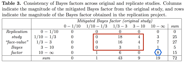
There are only 8 studies where both the bias mitigated original Bayes factors and the replication Bayes factors are above 10 (highlighted with the blue hexagon). That is, both experiment attempts provide strong evidence. It may go without saying, but I’ll say it anyway: These are the ideal cases. 

(The prior distribution for all Bayes factors is a normal distribution with mean of zero and variance of one. All the code is online HERE if you’d like to see how different priors change the result; our sensitivity analysis didn’t reveal any major dependencies on the exact prior used.)

The majority of studies (46/72) have both bias mitigated original and replication Bayes factors in the 1/10< BF <10 range (highlighted with the red box). These are cases where both study attempts only yielded weak evidence.

Table3

Overall, both attempts for most studies provided only weak evidence. There is a silver/bronze/rusty-metal lining, in that when both study attempts obtain only weak Bayes factors, they are technically providing consistent amounts of evidence. But that’s still bad, because “consistency” just means that we are systematically gathering weak evidence!

Using our analysis, no studies provided strong evidence that favored the null  hypothesis in either the original or replication.

It is interesting to consider the cases where one study attempt found strong evidence but another did not. I’ve highlighted these cases in blue in the table below. What can explain this?

Table3

One might be tempted to manufacture reasons that explain this pattern of results, but before you do that take a look at the figure below. We made this figure to highlight one common aspect of all study attempts that find weak evidence in one attempt and strong evidence in another: Differences in sample size. In all cases where the replication found strong evidence and the original study did not, the replication attempt had the larger sample size. Likewise, whenever the original study found strong evidence and the replication did not, the original study had a larger sample size.

RPP

Figure 2. Evidence resulting from replicated studies plotted against evidence resulting from the original publications. For the original publications, evidence for the alternative hypothesis was calculated taking into account the possibility of publication bias. Small crosses indicate cases where neither the replication nor the original gave strong evidence. Circles indicate cases where one or the other gave strong evidence, with the size of each circle proportional to the ratio of the replication sample size to the original sample size (a reference circle appears in the lower right). The area labeled ‘replication uninformative’ contains cases where the original provided strong evidence but the replication did not, and the area labeled ‘original uninformative’ contains cases where the reverse was true. Two studies that fell beyond the limits of the figure in the top right area (i.e., that yielded extremely large Bayes factors both times) and two that fell above the top left area (i.e., large Bayes factors in the replication only) are not shown. The effect that relative sample size has on Bayes factor pairs is shown by the systematic size difference of circles going from the bottom right to the top left. All values in this figure can be found in S1 Table.

Abridged conclusion (read the paper for more! More what? Nuance, of course. Bayesians are known for their nuance…)

Even when taken at face value, the original studies frequently provided only weak evidence when analyzed using Bayes factors (i.e., BF < 10), and as you’d expect this already small amount of evidence shrinks even more when you take into account the possibility of publication bias. This has a few nasty implications. As we say in the paper,

In the likely event that [the original] observed effect sizes were inflated … the sample size recommendations from prospective power analysis will have been underestimates, and thus replication studies will tend to find mostly weak evidence as well.

According to our analysis, in which a whopping 57 out of 72 replications had 1/10 < BF < 10, this appears to have been the case.

We also should be wary of claims about hidden moderators. We put it like this in the paper,

The apparent discrepancy between the original set of results and the outcome of the Reproducibility Project can be adequately explained by the combination of deleterious publication practices and weak standards of evidence, without recourse to hypothetical hidden moderators.

Of course, we are not saying that hidden moderators could not have had an influence on the results of the RPP. The statement is merely that we can explain the results reasonably well without necessarily bringing hidden moderators into the discussion. As Laplace would say: We have no need of that hypothesis.

So to sum up,

From a Bayesian reanalysis of the Reproducibility Project: Psychology, we conclude that one reason many published effects fail to replicate appears to be that the evidence for their existence was unacceptably weak in the first place.

With regard to interpretation of results — I will include the same disclaimer here that we provide in the paper:

It is important to keep in mind, however, that the Bayes factor as a measure of evidence must always be interpreted in the light of the substantive issue at hand: For extraordinary claims, we may reasonably require more evidence, while for certain situations—when data collection is very hard or the stakes are low—we may satisfy ourselves with smaller amounts of evidence. For our purposes, we will only consider Bayes factors of 10 or more as evidential—a value that would take an uninvested reader from equipoise to a 91% confidence level. Note that the Bayes factor represents the evidence from the sample; other readers can take these Bayes factors and combine them with their own personal prior odds to come to their own conclusions.

All of the results are tabulated in the supplementary materials (HERE) and the code is on github (CODE HERE).


More disclaimers, code, and differences from the old reanalysis

Disclaimer:

All of the results are tabulated in a table in the supplementary information (link), and MATLAB code to reproduce the results and figures is provided online (CODE HERE). When interpreting these results, we use a Bayes factor threshold of 10 to represent strong evidence. If you would like to see how the results change when using a different threshold, all you have to do is change the code in line 118 of the ‘bbc_main.m’ file to whatever thresholds you prefer.

#######

Important note: The function to calculate the mitigated Bayes factors is a prototype and is not robust to misuse. You should not use it unless you know what you are doing!

#######

A few differences between this paper and an old reanalysis:

A few months back I posted a Bayesian reanalysis of the Reproducibility Project: Psychology, in which I calculated replication Bayes factors for the RPP studies. This analysis took the posterior distribution from the original studies as the prior distribution in the replication studies to calculate the Bayes factor. So in that calculation, the hypotheses being compared are: H_0 “There is no effect” vs. H_A “The effect is close to that found by the original study.” It also did not take into account publication bias.

This is important: The published reanalysis is very different from the one in the first blog post.

Since the posterior distributions from the original studies were usually centered on quite large effects, the replication Bayes factors could fall in a wide range of values. If a replication found a moderately large effect, comparable to the original, then the Bayes factor would very largely favor H_A. If the replication found a small-to-zero effect (or an effect in the opposite direction), the Bayes factor would very largely favor H_0. If the replication found an effect in the middle of the two hypotheses, then the Bayes factor would be closer to 1, meaning the data fit both hypotheses equally bad. This last case happened when the replications found effects in the same direction as the original studies but of smaller magnitude.

These three types of outcomes happened with roughly equal frequency; there were lots of strong replications (big BF favoring H_A), lots of strong failures to replicate (BF favoring H_0), and lots of ambiguous results (BF around 1).

The results in this new reanalysis are not as extreme because the prior distribution for H_A is centered on zero, which means it makes more similar predictions to H_0 than the old priors. Whereas roughly 20% of the studies in the first reanalysis were strongly in favor of H_0 (BF>10), that did not happen a single time in the new reanalysis. This new analysis also includes the possibility of a biased publication processes, which can have a large effect on the results.

We use a different prior so we get different results. Hence the Jeffreys quote at the top of the page.


The next steps: Jerome Cornfield and sequential analysis

This is equivalent to saying that if the application of a principle to given evidence leads to an absurdity then the evidence must be discarded. It is reminiscent of the heavy smoker, who, worried by the literature relating smoking to lung cancer, decided to give up reading.

— Cornfield, 1966 (pdf link)

The next steps series intro:

After the great response to the eight easy steps paper we posted, I have decided to start a recurring series, where each week I highlight one of the papers that we included in the appendix of the paper. The format will be short and simple: I will give a quick summary of the paper while sharing a few excerpts that I like. If you’ve read our eight easy steps paper and you’d like to follow along on this extension, I think a pace of one paper per week is a perfect way to ease yourself into the Bayesian sphere. At the end of the post I will list a few suggestions for the next entry, so vote in the comments or on twitter (@alxetz) for which one you’d like next.


Sequential trials, sequential analysis and the likelihood principle

Theoretical focus, low difficulty

Cornfield (1966) begins by posing a question:

Do the conclusions to be drawn from any set of data depend only on the data or do they depend also on the stopping rule which led to the data? (p. 18)

The purpose of his paper is to discuss this question and explore the implications of answering “yes” versus “no.” This paper is a natural followup to entries one and three in the eight easy steps paper.

If you have read the eight easy steps paper (or at least the first and third steps), you’ll know that the answer to the above question for classical statistics is “yes”, while the answer for Bayesian statistics is “no.”

Cornfield introduces a concepts he calls the “α-postulate,” which states,

All hypotheses rejected at the same critical level [i.e., p<.05] have equal amounts of evidence against them. (p. 19)

Through a series of examples, Cornfield shows that the α-postulate appears to be false.

Cornfield then introduces a concept called the likelihood principle, which comes up in a few of the eight easy steps entries. The likelihood principle says that the likelihood function contains all of the information relevant to the evaluation of statistical evidence. Other facets of the data that do not factor into the likelihood function are irrelevant to the evaluation of the strength of the statistical evidence.

He goes on to show how subscription to the likelihood principle minimizes a linear combination of type-I (α) and type-II (β) error rates, as opposed to the Neyman-Pearson procedure that minimizes type-II error rates (i.e., maximizes power) for a fixed type-I error rate (usually 5%).

Thus, if instead of minimizing β for a given α, we minimize [their linear combination], we must come to the same conclusion for all sample points which have the same likelihood function, no matter what the design. (p. 21)


A few choice quotes

page 19 (emphasis added):

The following example will be recognized by statisticians with consulting experience as a simplified version of a very common situation. An experimenter, having made n observations in the expectation that they would permit the rejection of a particular hypothesis, at some predesignated significance level, say .05, finds that he has not quite attained this critical level. He still believes that the hypothesis is false and asks how many more observations would be required to have reasonable certainty of rejecting the hypothesis if the means observed after n observations are taken as the true values. He also makes it clear that had the original n observations permitted rejection he would simply have published his findings. Under these circumstances it is evident that there is no amount of additional observation, no matter how large, which would permit rejection at the .05 level. If the hypothesis being tested is true, there is a .05 chance of its having been rejected after the first round of observations. To this chance must be added the probability of rejecting after the second round, given failure to reject after the first, and this increases the total chance of erroneous rejection to above .05. In fact … no amount of additional evidence can be collected which would provide evidence against the hypothesis equivalent to rejection at the P =.05 level

page 19-20 (emphasis added):

I realize, of course, that practical people tend to become impatient with counter-examples of this type. Quite properly they regard principles as only approximate guides to practice, and not as prescriptions that must be literally followed even when they lead to absurdities. But if one is unwilling to be guided by the α-postulate in the examples given, why should he be any more willing to accept it when analyzing sequential trials? The biostatistician’s responsibility for providing biomedical scientists with a satisfactory explication of inference cannot, in my opinion, be satisfied by applying certain principles when he agrees with their consequences and by disregarding them when he doesn’t.

page 22 (emphasis added):

The stopping rule is this: continue observations until a normal mean differs from the hypothesized value by k standard errors, at which point stop. It is certain, using the rule, that one will eventually differ from the hypothesized value by at least k standard errors even when the hypothesis is true. … The Bayesian viewpoint of the example is as follows. If one is seriously concerned about the probability that a stopping rule will certainly result in the rejection of a true hypothesis, it must be because some possibility of the truth of the hypothesis is being entertained. In that case it is appropriate to assign a non-zero prior probability to the hypothesis. If this is done, differing from the hypothesized value by k standard errors will not result in the same posterior probability for the hypothesis for all values of n. In fact for fixed k the posterior probability of the hypothesis monotonically approaches unity as n increases, no matter how small the prior probability assigned, so long as it is non-zero, and how large the k, so long as it is finite. Differing by k standard errors does not therefore necessarily provide any evidence against the hypothesis and disregarding the stopping rule does not lead to an absurd conclusion. The Bayesian viewpoint thus indicates that the hypothesis is certain to be erroneously rejected-not because the stopping rule was disregarded-but because the hypothesis was assigned zero prior probability and that such assignment is inconsistent with concern over the possibility that the hypothesis will certainly be rejected when true.


Vote for the next entry:

  1. Edwards, Lindman, and Savage (1963) — Bayesian Statistical Inference for Psychological Research (pdf)
  2. Rouder (2014) — Optional Stopping: No Problem for Bayesians (pdf)
  3. Gallistel (2009) — The Importance of Proving the Null (pdf)
  4. Berger and Delampady (1987) — Testing Precise Hypotheses (pdf)


Understanding Bayes: How to become a Bayesian in eight easy steps

How to become a Bayesian in eight easy steps: An annotated reading list

(TLDR: We wrote an annotated reading list to get you started in learning Bayesian statistics. Published version. Researchgate. PsyArxiv.)

It can be hard to know where to start when you want to learn about Bayesian statistics. I am frequently asked to share my favorite introductory resources to Bayesian statistics, and my go-to answer has been to share a dropbox folder with a bunch of PDFs that aren’t really sorted or cohesive. In some sense I was acting as little more than a glorified Google Scholar search bar.

It seems like there is some tension out there with regard to Bayes, in that many people want to know more about it, but when they pick up, say, Andrew Gelman and colleagues’ Bayesian Data Analysis they get totally overwhelmed. And then they just think, “Screw this esoteric B.S.” and give up because it doesn’t seem like it is worth their time or effort.

I think this happens a lot. Introductory Bayesian texts usually assume a level of training in mathematical statistics that most researchers simply don’t have time (or otherwise don’t need) to learn. There are actually a lot of accessible Bayesian resources out there that don’t require much math stat background at all, but it just so happens that they are not consolidated anywhere so people don’t necessarily know about them.

Enter the eight step program

Beth Baribault, Peter Edelsbrunner (@peter1328), Fabian Dablander (@fdabl), Quentin Gronau, and I have just finished a new paper that tries to remedy this situation, titled, “How to become a Bayesian in eight easy steps: An annotated reading list.” We were invited to submit this paper for a special issue on Bayesian statistics for Psychonomic Bulletin and Review. Each paper in the special issue addresses a specific question we often hear about Bayesian statistics, and ours was the following:

I am a reviewer/editor handling a manuscript that uses Bayesian methods; which articles should I read to get a quick idea of what that means?

So the paper‘s goal is not so much to teach readers how to actually perform Bayesian data analysis — there are other papers in the special issue for that — but to facilitate readers in their quest to understand basic Bayesian concepts. We think it will serve as a nice introductory reading list for any interested researcher.

The format of the paper is straightforward. We highlight eight papers that had a big impact on our own understanding of Bayesian statistics, as well as short descriptions of an additional 28 resources in the Further reading appendix. The first four papers are focused on theoretical introductions, and the second four have a slightly more applied focus.

We also give every resource a ranking from 1–9 on two dimensions: Focus (theoretical vs. applied) and Difficulty (easy vs. hard). We tried to provide a wide range of resources, from easy applications (#14: Wagenmakers, Lee, and Morey’s “Bayesian benefits for the pragmatic researcher”) to challenging theoretical discussions (#12: Edwards, Lindman and Savage’s “Bayesian statistical inference for psychological research”) and others in between.

The figure below (Figure A1, available on the last page of the paper) summarizes our rankings:

Readinglist.png

The emboldened numbers (1–8) are the papers that we’ve commented on in detail, numbers in light text (9–30) are papers we briefly describe in the appendix, and the italicized numbers (31–36) are our recommended introductory books (also listed in the appendix).

This is how we chose to frame the paper,

Overall, the guide is designed such that a researcher might be able to read all eight of the highlighted articles and some supplemental readings within a few days. After readers acquaint themselves with these sources, they should be well-equipped both to interpret existing research and to evaluate new research that relies on Bayesian methods.

The list

Here’s the list of papers we chose to cover in detail:

  1.  Lindley (1993): The analysis of experimental data: The appreciation of tea and wine. PDF.
  2. Kruschke (2015, chapter 2): Introduction: Credibility, models, and parameters. Available on the DBDA website.
  3. Dienes (2011): Bayesian versus orthodox statistics: Which side are you on? PDF.
  4. Rouder, Speckman, Sun, Morey, & Iverson (2009): Bayesian t tests for accepting and rejecting the null hypothesis. PDF.
  5. Vandekerckhove, Matzke, & Wagenmakers (2014): Model comparison and the principle of parsimony. PDF.
  6. van de Schoot, Kaplan, Denissen, Asendorpf, Neyer, & Aken (2014): A gentle introduction to Bayesian analysis: Applications to developmental research. PDF.
  7. Lee and Vanpaemel (from the same special issue): Determining priors for cognitive models. PDF.
  8. Lee (2008): Three case studies in the Bayesian analysis of cognitive models. PDF.

You’ll have to check out the paper to see our commentary and to find out what other articles we included in the Further reading appendix. We provide urls (web archived when possible; archive.org/web/) to PDFs of the eight main papers (except #2, that’s on the DBDA website), and wherever possible for the rest of the resources (some did not have free copies online; see the References).

I thought this was a fun paper to write, and if you think you might want to learn some Bayesian basics I hope you will consider reading it.

Oh, and I should mention that we wrote the whole paper collaboratively on Overleaf.com. It is a great site that makes it easy to get started using LaTeX, and I highly recommend trying it out.

This is the fifth post in the Understanding Bayes series. Until next time,

bill-murray-youre-awesome