Today on Twitter there was some chatting about one-sided p-values. Daniel Lakens thinks that by 2018 we’ll see a renaissance of one-sided p-values due to the advent of preregistration. There was a great conversation that followed Daniel’s tweet, so go click the link above and read it and we’ll pick this back up once you do.
Okay.
As you have seen, and is typical of discussions around p-values in general, the question of evidence arises. How do one-sided p-values relate to two-sided p-values as measures of statistical evidence? In this post I will argue that thinking through the logic of one-sided p-values highlights a true illogic of significance testing. This example is largely adapted from Royall’s 1997 book.
The setup
The idea behind Fisher’s significance tests goes something like this. We have a hypothesis that we wish to find evidence against. If the evidence is strong enough then we can reject this hypothesis. I will use the binomial example because it lends itself to good storytelling, but this works for any test.
Premise A: Say I wish to determine if my coin is unfair. That is, I want to reject the hypothesis, H1, that the probability of heads is equal to ½. This is a standard two-sided test. If I flip my coin a few times and observe x heads, I can reject H1 (at level α) if the probability of obtaining x or more heads is less than α/2. If my α is set to the standard level, .05, then I can reject H1 if Pr(x or more heads) ≤ .025. In this framework, I have strong evidence that the probability of heads is not equal to ½ if my p-value is lower than .025. That is, I can claim (at level α) that the probability of heads is either greater than ½ or less than ½ (proposition A).
Premise B: If I have some reason to think the coin might be biased one way or the other, say there is a kid on the block with a coin biased to come up heads more often than not, then I might want to use a one-sided test. In this test, the hypothesis to be rejected, H2, is that the probability of heads is less than or equal to ½. In this case I can reject H2 (at level α) if the probability of obtaining x or more heads is less than α. If my α is set to the standard level again, .05, then I can reject H2 if Pr(x or more heads) < .05. Now I have strong evidence that the probability of heads is not equal to ½, nor is it less than ½, if my p-value is less than .05. That is, I can claim (again at level α) that the probability of heads is greater than ½. (proposition B).
As you can see, proposition B is a stronger logical claim than proposition A. Saying that my car is faster than your car is making a stronger claim than saying that my car is either faster or slower than your car.
The paradox
If I obtain a result x, such that α/2 < Pr(x or more heads) < α, (e.g., .025 < p < .05), then I have strong evidence for the conclusion that the probability of heads is greater than ½ (see proposition B). But at the same time I do not have strong evidence for the conclusion that the probability of heads is > ½ or < ½ (see proposition A).
I have defied the rules of logic. I have concluded the stronger proposition, probability of heads > ½, but I cannot conclude the weaker proposition, probability of heads > ½ or < ½. As Royall (1997, p. 77) would say, if the evidence justifies the conclusion that the probability of heads is greater than ½ then surely it justifies the weaker conclusion that the probability of heads is either > ½ or < ½.
Should we use one-sided p-values?
Go ahead, I can’t stop you. But be aware that if you try to interpret p-values, either one- or two-sided, as measures of statistical (logical) evidence then you may find yourself in a p-value paradox.
References and further reading:
Royall, R. (1997). Statistical evidence: A likelihood paradigm (Vol. 71). CRC press. Chapter 3.7.
[This post has been updated and turned into a paper to be published in AMPPS]
Much of the discussion in psychology surrounding Bayesian inference focuses on priors. Should we embrace priors, or should we be skeptical? When are Bayesian methods sensitive to specification of the prior, and when do the data effectively overwhelm it? Should we use context specific prior distributions or should we use general defaults? These are all great questions and great discussions to be having.
One thing that often gets left out of the discussion is the importance of the likelihood. The likelihood is the workhorse of Bayesian inference. In order to understand Bayesian parameter estimation you need to understand the likelihood. In order to understand Bayesian model comparison (Bayes factors) you need to understand the likelihood and likelihood ratios.
What is likelihood?
Likelihood is a funny concept. It’s not a probability, but it is proportional to a probability. The likelihood of a hypothesis (H) given some data (D) is proportional to the probability of obtaining D given that H is true, multiplied by an arbitrary positive constant (K). In other words, L(H|D) = K · P(D|H). Since a likelihood isn’t actually a probability it doesn’t obey various rules of probability. For example, likelihood need not sum to 1.
A critical difference between probability and likelihood is in the interpretation of what is fixed and what can vary. In the case of a conditional probability, P(D|H), the hypothesis is fixed and the data are free to vary. Likelihood, however, is the opposite. The likelihood of a hypothesis, L(H|D), conditions on the data as if they are fixed while allowing the hypotheses to vary.
The distinction is subtle, so I’ll say it again. For conditional probability, the hypothesis is treated as a given and the data are free to vary. For likelihood, the data are a given and the hypotheses vary.
The Likelihood Axiom
Edwards (1992, p. 30) defines the Likelihood Axiom as a natural combination of the Law of Likelihood and the Likelihood Principle.
The Law of Likelihood states that “within the framework of a statistical model, a particular set of data supports one statistical hypothesis better than another if the likelihood of the first hypothesis, on the data, exceeds the likelihood of the second hypothesis” (Emphasis original. Edwards, 1992, p. 30).
In other words, there is evidence for H1 vis-a-vis H2 if and only if the probability of the data under H1 is greater than the probability of the data under H2. That is, D is evidence for H1 over H2 if P(D|H1) > P(D|H2). If these two probabilities are equivalent, then there is no evidence for either hypothesis over the other. Furthermore, the strength of the statistical evidence for H1 over H2 is quantified by the ratio of their likelihoods, L(H1|D)/L(H2|D) (which again is proportional to P(D|H1)/P(D|H2) up to an arbitrary constant that cancels out).
The Likelihood Principle states that the likelihood function contains all of the information relevant to the evaluation of statistical evidence. Other facets of the data that do not factor into the likelihood function are irrelevant to the evaluation of the strength of the statistical evidence (Edwards, 1992, p. 30; Royall, 1997, p. 22). They can be meaningful for planning studies or for decision analysis, but they are separate from the strength of the statistical evidence.
Likelihoods are meaningless in isolation
Unlike a probability, a likelihood has no real meaning per se due to the arbitrary constant. Only by comparing likelihoods do they become interpretable, because the constant in each likelihood cancels the other one out. The easiest way to explain this aspect of likelihood is to use the binomial distribution as an example.
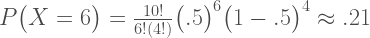
Suppose I flip a coin 10 times and it comes up 6 heads and 4 tails. If the coin were fair, p(heads) = .5, the probability of this occurrence is defined by the binomial distribution:
where x is the number of heads obtained, n is the total number of flips, p is the probability of heads, and
Substituting in our values we get
If the coin were a trick coin, so that p(heads) = .75, the probability of 6 heads in 10 tosses is:
To quantify the statistical evidence for the first hypothesis against the second, we simply divide one probability by the other. This ratio tells us everything we need to know about the support the data lends to one hypothesis vis-a-vis the other. In the case of 6 heads in 10 tosses, the likelihood ratio (LR) for a fair coin vs our trick coin is:
Translation: The data are 1.4 times as probable under a fair coin hypothesis than under this particular trick coin hypothesis. Notice how the first terms in each of the equations above, i.e., , are equivalent and completely cancel each other out in the likelihood ratio.
Same data. Same constant. Cancel out.
The first term in the equations above, , details our journey to obtaining 6 heads out of 10. If we change our journey (i.e., different sampling plan) then this changes the term’s value, but crucially, since it is the same term in both the numerator and denominator it always cancels itself out. In other words, the information contained in the way the data are obtained disappears from the function. Hence the irrelevance of the stopping rule to the evaluation of statistical evidence, which is something that makes bayesian and likelihood methods valuable and flexible.
If we leave out the first term in the above calculations, our numerator is L(.5) = 0.0009765625 and our denominator is L(.75) ≈ 0.0006952286. Using these values to form the likelihood ratio we get: 0.0009765625/0.0006952286 ≈ 1.4,as we should since the other terms simply cancelled out before.
Again I want to reiterate that the value of a single likelihood is meaningless in isolation; only in comparing likelihoods do we find meaning.
Looking at likelihoods
Likelihoods may seem overly restrictive at first. We can only compare 2 simple statistical hypotheses in a single likelihood ratio. But what if we are interested in comparing many more hypotheses at once? What if we want to compare all possible hypotheses at once?
In that case we can plot the likelihood function for our data, and this lets us ‘see’ the evidence in its entirety. By plotting the entire likelihood function we compare all possible hypotheses simultaneously. The Likelihood Principle tells us that the likelihood function encompasses all statistical evidence that our data can provide, so we should always plot this function along side our reported likelihood ratios.
Following the wisdom of Birnbaum (1962), “the “evidential meaning” of experimental results is characterized fully by the likelihood function” (as cited in Royall, 1997, p.25). So let’s look at some examples. The R script at the end of this post can be used to reproduce these plots, or you can use it to make your own plots. Play around with it and see how the functions change for different number of heads, total flips, and hypotheses of interest. See the instructions in the script for details.
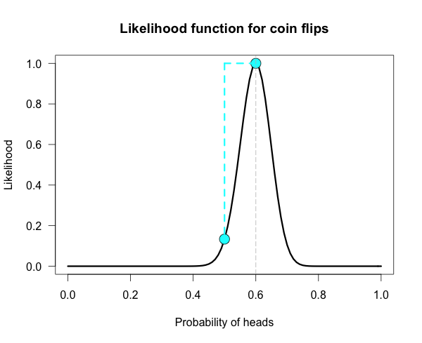
Below is the likelihood function for 6 heads in 10 tosses. I’ve marked our two hypotheses from before on the likelihood curve with blue dots. Since the likelihood function is meaningful only up to an arbitrary constant, the graph is scaled by convention so that the best supported value (i.e., the maximum) corresponds to a likelihood of 1.
The vertical dotted line marks the hypothesis best supported by the data. The likelihood ratio of any two hypotheses is simply the ratio of their heights on this curve. We can see from the plot that the fair coin has a higher likelihood than our trick coin.
How does the curve change if instead of 6 heads out of 10 tosses, we tossed 100 times and obtained 60 heads?
Our curve gets much narrower! How did the strength of evidence change for the fair coin vs the trick coin? The new likelihood ratio is L(.5)/L(.75) ≈ 29.9. Much stronger evidence!(footnote) However, due to the narrowing, neither of these hypothesized values are very high up on the curve anymore. It might be more informative to compare each of our hypotheses against the best supported hypothesis. This gives us two likelihood ratios: L(.6)/L(.5) ≈ 7.5 and L(.6)/L(.75) ≈ 224.
Here is one more curve, for when we obtain 300 heads in 500 coin flips.
Notice that both of our hypotheses look to be very near the minimum of the graph. Yet their likelihood ratio is much stronger than before. For this data the likelihood ratio L(.5)/L(.75) is nearly 24 million! The inherent relativity of evidence is made clear here: The fair coin was supported when compared to one particular trick coin. But this should not be interpreted as absolute evidence for the fair coin, because the likelihood ratio for the maximally supported hypothesis vs the fair coin, L(.6)/L(.5), is nearly 24 thousand!
We need to be careful not to make blanket statements about absolute support, such as claiming that the maximum is “strongly supported by the data”. Always ask, “Compared to what?” The best supported hypothesis will be only be weakly supported vs any hypothesis just before or just after it on the x-axis. For example, L(.6)/L(.61) ≈ 1.1, which is barely any support one way or the other. It cannot be said enough that evidence for a hypothesis must be evaluated in consideration with a specific alternative.
Connecting likelihood ratios to Bayes factors
Bayes factors are simple extensions of likelihood ratios. A Bayes factor is a weighted average likelihood ratio based on the prior distribution specified for the hypotheses. (When the hypotheses are simple point hypotheses, the Bayes factor is equivalent to the likelihood ratio.) The likelihood ratio is evaluated at each point of the prior distribution and weighted by the probability we assign that value. If the prior distribution assigns the majority of its probability to values far away from the observed data, then the average likelihood for that hypothesis is lower than one that assigns probability closer to the observed data. In other words, you get a Bayes boost if you make more accurate predictions. Bayes factors are extremely valuable, and in a future post I will tackle the hard problem of assigning priors and evaluating weighted likelihoods.
I hope you come away from this post with a greater knowledge of, and appreciation for, likelihoods. Play around with the R code and you can get a feel for how the likelihood functions change for different data and different hypotheses of interest.
(footnote) Obtaining 60 heads in 100 tosses is equivalent to obtaining 6 heads in 10 tosses 10 separate times. To obtain this new likelihood ratio we can simply multiply our ratios together. That is, raise the first ratio to the power of 10; 1.4^10 ≈ 28.9, which is just slightly off from the correct value of 29.9 due to rounding.
R Code
This file contains hidden or bidirectional Unicode text that may be interpreted or compiled differently than what appears below. To review, open the file in an editor that reveals hidden Unicode characters.
Learn more about bidirectional Unicode characters


 , are equivalent and completely cancel each other out in the likelihood ratio.