Understanding Bayes: How to cheat to get the maximum Bayes factor for a given p value

June 19, 2016June 19, 2016 Alex Etz Psychology, Statistics, Understanding Bayes Bayes, Bayes factor, hypothesis testing, Likelihood, probability, Psychology, statistical evidence, Statistics

OR less click-baity: What is the maximum Bayes factor you can get for a given p value? (Obvious disclaimer: Don’t cheat)

Starting to use and interpret Bayesian statistics can be hard at first. A recent recommendation that I like is from Zoltan Dienes and Neil Mclatchie, to “Report a B for every p.” Meaning, for every p value in the paper report a corresponding Bayes factor. This way the psychology community can start to build an intuition about how these two kinds of results can correspond. I think this is a great way to start using Bayes. And if as time goes on you want to flush those ps down the toilet, I won’t complain.

Researchers who start to report both Bayesian and frequentist results often go through a phase where they are surprised to find that their p<.05 results correspond to weak Bayes factors. In this Understanding Bayes post I hope to pump your intuitions a bit as to why this is the case. There is, in fact, an absolute maximum Bayes factor for a given p value. There are also other soft maximums it can achieve for different classes of prior distributions. And these maximum BFs may not be as high as you expect.

Absolute Maximum

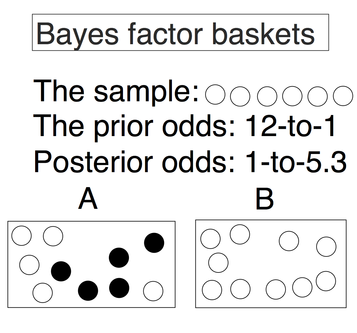
The reason for the absolute maximum is actually straightforward. The Bayes factor compares how accurately two or more competing hypotheses predict the observed data. Usually one of those hypotheses is a point null hypothesis, which says there is no effect in the population (however defined). The alternative can be anything you like. It could be a point hypothesis motivated by theory or that you take from previous literature (uncommon), or it can be a (half-)normal (or other) distribution centered on the null (more common), or anything else. In any case, the fact is that to achieve the absolute maximum Bayes factor for a given p value you have to cheat. In real life you can never reach the absolute maximum in a normal course of analysis so its only use is as a benchmark illustration.

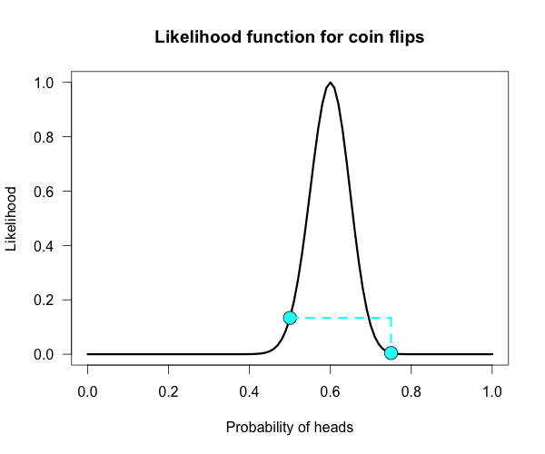
You have to make your alternative hypothesis the exact point hypothesis that maximizes the likelihood of the data. The likelihood function ranks all the parameter values by how well they predict the data, so if you make your point hypothesis equal to the mode of the likelihood function, it means that no other hypothesis or population parameter could make the data more likely. This illicit prior is known as the oracle prior, because it is the prior you would choose if you could see the result ahead of time. So in the figure below, the oracle prior would correspond to the high dot on the curve at the mode, and the null hypothesis is the lower dot on the curve. The Bayes factor is then just the ratio of these heights.

When you are doing a t-test, for example, the maximum of the likelihood function is simply the sample mean. So in this case, the oracle prior is a point hypothesis at exactly the sample mean. Let’s assume that we know the population SD=10, so we’re only interested in the population mean. We collect 100 participants and the sample mean we get is 1.96. Our z score in this case is

z = mean / standard error = 1.96 / (10/√100) = 1.96.

This means we obtain a p value of exactly .05. Publication and glory await us. But, in sticking with our B for every p mantra, we decide to calculate an oracle Bayes factor just to be complete. This can easily be done in R using the following 1 line of code:

dnorm(1.96, 1.96, 1)/dnorm(1.96, 0, 1)

And the answer you get is BF = 6.83. This is the absolute maximum Bayes factor you can possibly get for a p value that equals .05 in a t test (you get similar BFs for other types of tests). That is the amount of evidence that would bring a neutral reader who has prior probabilities of 50% for the null and 50% for the alternative to posterior probabilities of 12.8% for the null and 87.2% for the alternative. You might call that moderate evidence depending on the situation. For p of .01, this maximum increases to ~27.5, which is quite strong in most cases. But these values are for the best case ever, where you straight up cheat. When you can’t blatantly cheat the results are not so good.

Soft Maximum

Of course, nobody in their right mind would accept your analysis if you used an oracle prior. It is blatant cheating — but it gives a good benchmark. For p of .05 and the oracle prior, the best BF you can ever get is slightly less than 7. If you can’t blatantly cheat by using an oracle prior, the maximum Bayes factor you can get obviously won’t be as high. But it may surprise you how much smaller the maximum becomes if you decide to cheat more subtly.

The priors most people use for the alternative hypothesis in the Bayes factor are not point hypotheses, but distributed hypotheses. A common recommendation is a unimodal (i.e., one-hump) symmetric prior centered on the null hypothesis value. (There are times where you wouldn’t want to use a prior centered on the null value, but in those cases the maximum BF goes back to being the BF you get using an oracle prior.) I usually recommend using normal distribution priors, and JASP software uses a Cauchy distribution which is similar but with fatter tails. Most of the time the BFs you get are very similar.

So imagine that instead of using the blatantly cheating oracle prior, you use a subtle oracle prior. Instead of a point alternative at the observed mean, you use a normal distribution and pick the scale (i.e., the SD) of your prior to maximize the Bayes factor. There is a formula for this, but the derivation is very technical so I’ll let you read Berger and Sellke (1987, especially section 3) if you’re into that sort of torture.

It turns out, once you do the math, that when using a normal distribution prior the maximum Bayes factor you can get for a p value of .05 is BF = 2.1. That is the amount of evidence that would bring a neutral reader who has prior probabilities of 50% for the null and 50% for the alternative to posterior probabilities of 32% for the null and 68% for the alternative. Barely different! That is very weak evidence. The maximum normal prior BF corresponding to p of .01 is BF = 6.5. That is still hardly convincing evidence! You can find this bound for any t value you like (for any t greater than 1) using the R code below:

t = 1.96
maxBF = 1/(sqrt(exp(1))*t*exp(-t^2/2))

(You can get slightly different maximum values for different formulations of problem. Another form due to Sellke, Bayarri, & Berger [2001] is 1/[-e*p*ln(p)] for p<~.4, which for p=.05 returns BF = 2.45)

You might say, “Wait no I have a directional prediction, so I will use a half-normal prior that allows only positive values for the population mean. What is my maximum BF now?” Luckily the answer is simple: Just multiply the old maximum by:

2*(1 – p/2)

So for p of .05 and .01 the maximum 1-sided BFs are 4.1 and 13, respectively. (By the way, this trick works for converting most common BFs from 2- to 1-sided.)

Take home message

Do not be surprised if you start reporting Bayes factors and find that what you thought was strong evidence based on a p value of .05 or even .01 translates to a quite weak Bayes factor.

And I think this goes without saying, but don’t try to game your Bayes factors. We’ll know. It’s obvious. The best thing to do is use the prior distribution you find most reasonable for the problem at hand and then do a robustness check by seeing how much the conclusion you draw depends on the specific prior you choose. JASP software can do this for you automatically in many cases (e.g., for the Bayesian t-test; ps check out our official JASP tutorial videos!).

R code

The following is the R code to reproduce the figure, to find the max BF for oracle priors, and to find the max BF for subtle oracle priors. Tinker with it and see how your intuitions match the answers you get!

	#This is the code for Alexander Etz's blog at http://wp.me/p4sgtg-SQ

	#Code to make the figure and find max oracle BF for normal data
	maxL <- function(mean=1.96,se=1,h0=0){
	L1 <-dnorm(mean,mean,se)
	L2 <-dnorm(mean,h0,se)
	Ratio <- L1/L2
	curve(dnorm(x,mean,se), xlim = c(-2mean,2.5mean), ylab = "Likelihood", xlab = "Population mean", las=1,
	main = "Likelihood function for the mean", lwd = 3)
	points(mean, L1, cex = 2, pch = 21, bg = "cyan")
	points(h0, L2, cex = 2, pch = 21, bg = "cyan")
	lines(c(mean, h0), c(L1, L1), lwd = 3, lty = 2, col = "cyan")
	lines(c(h0, h0), c(L1, L2), lwd = 3, lty = 2, col = "cyan")
	return(Ratio) ## Returns the Bayes factor for oracle hypothesis vs null
	}

	#Code to find the max subtle oracle prior BF for normal data
	t = 1.96 #Critical value corresponding to the p value
	maxBF = 1/(sqrt(exp(1))texp(-t^2/2)) #Formula from Berger and Sellke 1987
	#multiply by 2*(1-p/2) if using a one-sided prior

view raw MaxBF.R hosted with ❤ by GitHub

The next steps: Jerome Cornfield and sequential analysis

February 21, 2016February 21, 2016 Alex Etz Article Review, Statistics Article Review, Bayes, Likelihood, probability, Statistics

This is equivalent to saying that if the application of a principle to given evidence leads to an absurdity then the evidence must be discarded. It is reminiscent of the heavy smoker, who, worried by the literature relating smoking to lung cancer, decided to give up reading.

— Cornfield, 1966 (pdf link)

The next steps series intro:

After the great response to the eight easy steps paper we posted, I have decided to start a recurring series, where each week I highlight one of the papers that we included in the appendix of the paper. The format will be short and simple: I will give a quick summary of the paper while sharing a few excerpts that I like. If you’ve read our eight easy steps paper and you’d like to follow along on this extension, I think a pace of one paper per week is a perfect way to ease yourself into the Bayesian sphere. At the end of the post I will list a few suggestions for the next entry, so vote in the comments or on twitter (@alxetz) for which one you’d like next.

Sequential trials, sequential analysis and the likelihood principle

Theoretical focus, low difficulty

Cornfield (1966) begins by posing a question:

Do the conclusions to be drawn from any set of data depend only on the data or do they depend also on the stopping rule which led to the data? (p. 18)

The purpose of his paper is to discuss this question and explore the implications of answering “yes” versus “no.” This paper is a natural followup to entries one and three in the eight easy steps paper.

If you have read the eight easy steps paper (or at least the first and third steps), you’ll know that the answer to the above question for classical statistics is “yes”, while the answer for Bayesian statistics is “no.”

Cornfield introduces a concepts he calls the “α-postulate,” which states,

All hypotheses rejected at the same critical level [i.e., p<.05] have equal amounts of evidence against them. (p. 19)

Through a series of examples, Cornfield shows that the α-postulate appears to be false.

Cornfield then introduces a concept called the likelihood principle, which comes up in a few of the eight easy steps entries. The likelihood principle says that the likelihood function contains all of the information relevant to the evaluation of statistical evidence. Other facets of the data that do not factor into the likelihood function are irrelevant to the evaluation of the strength of the statistical evidence.

He goes on to show how subscription to the likelihood principle minimizes a linear combination of type-I (α) and type-II (β) error rates, as opposed to the Neyman-Pearson procedure that minimizes type-II error rates (i.e., maximizes power) for a fixed type-I error rate (usually 5%).

Thus, if instead of minimizing β for a given α, we minimize [their linear combination], we must come to the same conclusion for all sample points which have the same likelihood function, no matter what the design. (p. 21)

A few choice quotes

page 19 (emphasis added):

The following example will be recognized by statisticians with consulting experience as a simplified version of a very common situation. An experimenter, having made n observations in the expectation that they would permit the rejection of a particular hypothesis, at some predesignated significance level, say .05, finds that he has not quite attained this critical level. He still believes that the hypothesis is false and asks how many more observations would be required to have reasonable certainty of rejecting the hypothesis if the means observed after n observations are taken as the true values. He also makes it clear that had the original n observations permitted rejection he would simply have published his findings. Under these circumstances it is evident that there is no amount of additional observation, no matter how large, which would permit rejection at the .05 level. If the hypothesis being tested is true, there is a .05 chance of its having been rejected after the first round of observations. To this chance must be added the probability of rejecting after the second round, given failure to reject after the first, and this increases the total chance of erroneous rejection to above .05. In fact … no amount of additional evidence can be collected which would provide evidence against the hypothesis equivalent to rejection at the P =.05 level

page 19-20 (emphasis added):

I realize, of course, that practical people tend to become impatient with counter-examples of this type. Quite properly they regard principles as only approximate guides to practice, and not as prescriptions that must be literally followed even when they lead to absurdities. But if one is unwilling to be guided by the α-postulate in the examples given, why should he be any more willing to accept it when analyzing sequential trials? The biostatistician’s responsibility for providing biomedical scientists with a satisfactory explication of inference cannot, in my opinion, be satisfied by applying certain principles when he agrees with their consequences and by disregarding them when he doesn’t.

page 22 (emphasis added):

The stopping rule is this: continue observations until a normal mean differs from the hypothesized value by k standard errors, at which point stop. It is certain, using the rule, that one will eventually differ from the hypothesized value by at least k standard errors even when the hypothesis is true. … The Bayesian viewpoint of the example is as follows. If one is seriously concerned about the probability that a stopping rule will certainly result in the rejection of a true hypothesis, it must be because some possibility of the truth of the hypothesis is being entertained. In that case it is appropriate to assign a non-zero prior probability to the hypothesis. If this is done, differing from the hypothesized value by k standard errors will not result in the same posterior probability for the hypothesis for all values of n. In fact for fixed k the posterior probability of the hypothesis monotonically approaches unity as n increases, no matter how small the prior probability assigned, so long as it is non-zero, and how large the k, so long as it is finite. Differing by k standard errors does not therefore necessarily provide any evidence against the hypothesis and disregarding the stopping rule does not lead to an absurd conclusion. The Bayesian viewpoint thus indicates that the hypothesis is certain to be erroneously rejected-not because the stopping rule was disregarded-but because the hypothesis was assigned zero prior probability and that such assignment is inconsistent with concern over the possibility that the hypothesis will certainly be rejected when true.

Vote for the next entry:

Edwards, Lindman, and Savage (1963) — Bayesian Statistical Inference for Psychological Research (pdf)
Rouder (2014) — Optional Stopping: No Problem for Bayesians (pdf)
Gallistel (2009) — The Importance of Proving the Null (pdf)
Berger and Delampady (1987) — Testing Precise Hypotheses (pdf)

Slides: “Bayesian statistical concepts: A gentle introduction”

November 8, 2015November 12, 2015 Alex Etz Presentations, Statistics Bayes, Likelihood, probability, statistical evidence, Statistics

I recently gave a talk in Bielefeld, Germany with the title “Bayesian statistical concepts: A gentle introduction.” I had a few people ask for the slides so I figured I would post them here. If you are a regular reader of this blog, it should all look pretty familiar. It was a mesh of a couple of my Understanding Bayes posts, combining “A look at the Likelihood” and the most recent one, “Evidence vs. Conclusions.” The main goal was to give the audience an appreciation for the comparative nature of Bayesian statistical evidence, as well as demonstrate how evidence in the sample has to be interpreted in the context of the specific problem. I didn’t go into Bayes factors or posterior estimation because I promised that it would be a simple and easy talk about the basic concepts.

I’m very grateful to JP de Ruiter for inviting me out to Bielefeld to give this talk, in part because it was my first talk ever! I think it went well enough, but there are a lot of things I can improve on; both in terms of slide content and verbal presentation. JP is very generous with his compliments, and he also gave me a lot of good pointers to incorporate for the next time I talk Bayes.

The main narrative of my talk was that we were to draw candies from one of two possible bags and try to figure out which bag we were drawing from. After each of the slides where I proposed the game I had a member of the audience actually come up and play it with me. The candies, bags, and cards were real but the bets were hypothetical. It was a lot of fun. 🙂

Here is a picture JP took during the talk.

Here are the slides. (You can download a pdf copy from here.)

Understanding Bayes: Evidence vs. Conclusions

November 1, 2015November 2, 2015 Alex Etz Statistics, Understanding Bayes Bayes, Bayes factor, Conclusions, Likelihood

In this installment of Understanding Bayes I want to discuss the nature of Bayesian evidence and conclusions. In a previous post I focused on Bayes factors’ mathematical structure and visualization. In this post I hope to give some idea of how Bayes factors should be interpreted in context. How do we use the Bayes factor to come to a conclusion?

How to calculate a Bayes factor

I’m going to start with an example to show the nature of the Bayes factor. Imagine I have 2 baskets with black and white balls in them. In basket A there are 5 white balls and 5 black balls. In basket B there are 10 white balls. Other than the color, the balls are completely indistinguishable. Here’s my advanced high-tech figure depicting the problem.

You choose a basket and bring it to me. The baskets aren’t labeled so I can’t tell by their appearance which one you brought. You tell me that in order to figure out which basket I have, I am allowed to take a ball out one at a time and then return it and reshuffle the balls around. What outcomes are possible here? In this case it’s super simple: I can either draw a white ball or a black ball.

If I draw a black ball I immediately know I have basket A, since this is impossible in basket B. If I draw a white ball I can’t rule anything out, but drawing a white ball counts as evidence for basket B over basket A. Since the white ball occurs with probability 1 if I have basket B, and probability .5 if I have basket A, then due to what is known as the Likelihood Axiom, I have evidence for basket B over basket A by a factor of 2. See this post for a refresher on likelihoods, including the concepts such as the law of likelihood and the likelihood principle. The short version is that observations count as evidence for basket B over basket A if they are more probable given basket B than basket A.

I continue to sample, and end up with this set of observations: {W, W, W, W, W, W}. Each white ball that I draw counts as evidence of 2 for basket B over basket A, so my evidence looks like this: {2, 2, 2, 2, 2, 2}. Multiply them all together and my total evidence for B over A is 2^6, or 64. This interpretation is simple: The total accumulated data are, all together, 64 times more probable under basket B than basket A. This number represents a simple Bayes factor, or likelihood ratio.

How to interpret a Bayes factor

In one sense, the Bayes factor always has the same interpretation in every problem: It is a ratio formed by the probability of the data under each hypothesis. It’s all about prediction. The bigger the Bayes factor the more one hypothesis outpredicted the other.

But in another sense the interpretation, and our reaction, necessarily depends on the context of the problem, and that is represented by another piece of the Bayesian machinery: The prior odds. The Bayes factor is the factor by which the data shift the balance of evidence from one hypothesis to another, and thus the amount by which the prior odds shift to posterior odds.

Imagine that before you brought me one of the baskets you told me you would draw a card from a standard, shuffled deck of cards. You have a rule: Bring me basket B if the card drawn is a black suit and bring basket A if it is a red suit. You pick a card and, without telling me what it was, bring me a basket. Which basket did you bring me? What information do I have about the basket before I get to draw a sample from it?

I know that there is a 50% chance that you choose a black card, so there is a 50% chance that you bring me basket B. Likewise for basket A. The prior probabilities in this scenario are 50% for each basket, so the prior odds for basket A vs basket B are 1-to-1. (To calculate odds you just divide the probability of one hypothesis by the other.)

Let’s say we draw our sample and get the same results as before: {W, W, W, W, W, W}. The evidence is the same: {2, 2, 2, 2, 2, 2} and the Bayes factor is the same, 2^6=64. What do we conclude from this? Should we conclude we have basket A or basket B?

The conclusion is not represented by the Bayes factor, but by the posterior odds. The Bayes factor is just one piece of the puzzle, namely the evidence contained in our sample. In order to come to a conclusion the Bayes factor has to be combined with the prior odds to obtain posterior odds. We have to take into account the information we had before we started sampling. I repeat: The posterior odds are where the conclusion resides. Not the Bayes factor.

Posterior odds (or probabilities) and conclusions

In the example just given, the posterior odds happen to equal the Bayes factor. Since the prior odds were 1-to-1, we multiply by the Bayes factor of 1-to-64, to obtain posterior odds of 1-to-64 favoring basket B. This means that, when these are the only two possible baskets, the probability of basket A has shrunk from 50% to 2% and the probability of basket B has grown from 50% to 98%. (To convert odds to probabilities divide the odds by odds+1.) This is the conclusion, and it necessarily depends on the prior odds we assign.

Say you had a different rule for picking the baskets. Let’s say that this time you draw a card and bring me basket B if you draw a King (of any suit) and you bring me basket A if you draw any other card. Now the prior odds are 48-to-4, or 12-to-1, in favor of basket A.

The data from our sample are the same, {W, W, W, W, W, W}, and so is the Bayes factor, 2^6= 64. The conclusion is qualitatively the same, with posterior odds of 1-to-5.3 that favor basket B. This means that, again when considering these as the only two possible baskets, the probability of basket A has been shrunk from 92% to 16% and the probability of basket B has grown from 8% to 84%. The Bayes factor is the same, but we are less confident in our conclusion. The prior odds heavily favored basket A, so it takes more evidence to overcome this handicap and reach as strong a conclusion as before.

What happens when we change the rule once again: Bring me basket B if you draw a King of Hearts and basket A if you draw any other card. Now the prior odds are 51-to-1 in favor of basket A. The data are the same again, and the Bayes factor is still 64. Now the posterior odds are 1-to-1.3 in favor of basket B. This means that the probability of basket A has been shrunk from 98% to 43% and the probability of basket B has grown from 2% to 57%. The evidence, and the Bayes factor, is exactly the same — but the conclusion is totally ambiguous.

Evidence vs. Conclusions

In each case I’ve considered, the evidence has been exactly the same: 6 draws, all white. As a corollary to the discussion above, if you try to come to conclusions based only on the Bayes factor then you are implicitly assuming prior odds of 1-to-1. I think this is unreasonable in most circumstances. When someone looks at a medium-to-large Bayes factor in a study claiming “sadness impairs color perception” (or some other ‘cute’ metaphor study published in Psych Science) and thinks, “I don’t buy this,” they are injecting their prior odds into the equation. Their implicit conclusion is: “My posterior odds for this study are not favorable.” This is the conclusion. The Bayes factor is not the conclusion.

Many studies follow-up on earlier work, so we might give favorable prior odds; thus, when we see a Bayes factor of 5 or 10 we “buy what the study is selling,” so to speak. Or the study might be testing something totally new, so we might give unfavorable prior odds; thus, when we see a Bayes factor of 5 or 10 we remain skeptical. This is just another way of saying that we may reasonably require more evidence for extraordinary claims.

When to stop collecting data

It also follows from the above discussion that sometimes enough is enough. What I mean is that sometimes the conclusion for any reasonable prior odds assignment is strong enough that collecting more data is not worth the time, money, or energy. In the Bayesian framework the stopping rules don’t affect the Bayes factor, and subsequently they don’t affect the posterior odds. Take the second example above, where you gave me basket B if you drew any King. I had prior odds of 12-to-1 in favor of basket A, drew 6 white balls in a row, and ended up with 1-to-5.3 posterior odds in favor of basket B. This translated to a posterior probability of 84% for basket B. If I draw 2 more balls and they are both white, my Bayes factor increases to 2^8=256 (and this should not be corrected for multiple comparisons or so-called “topping up”). My posterior odds increase to roughly 1-to-21 in favor of basket B, and the probability for basket B shoots up from 84% to 99%. I would say that’s enough data for me to make a firm conclusion. But someone else might have other relevant information about the problem I’m studying, and they can come to a different conclusion.

Conclusions are personal

There’s no reason another observer has to come to the same conclusion as me. She might have talked to you and you told her that you actually drew three cards (with replacement and reshuffle) and that you would only have brought me basket B if you drew three kings in a row. She has different information than I do, so naturally she has different prior odds (1728-to-1 in favor of basket A). She would come to a different conclusion than I would, namely that I was actually probably sampling from basket A — her posterior odds are roughly 7-to-1 in favor of basket A. We use the same evidence, a Bayes factor of 2^8=256, but come to different conclusions.

Conclusions are personal. I can’t tell you what to conclude because I don’t know all the information you have access to. But I can tell you what the evidence is, and you can use that to come to your own conclusion. In this post I used a mechanism to generate prior odds that are intuitive and obvious, but we come to our scientific judgments through all sorts of ways that aren’t always easily expressed or quantified. The idea is the same however you come to your prior odds: If you’re skeptical of a study that has a large Bayes factor, then you assigned it strongly unfavorable prior odds.

This is why I, and other Bayesians, advocate for reporting the Bayes factor in experiments. It is not because it tells someone what to conclude from the study, but that it lets them take the information contained in your data to come to their own conclusion. When you report your own Bayes factors for your experiments, in your discussion you might consider how people with different prior odds will react to your evidence. If your Bayes factor is not strong enough to overcome a skeptic’s prior odds, then you may consider collecting more data until it is. If you’re out of resources and the Bayes factor is not strong enough to overcome the prior odds of a moderate skeptic, then there is nothing wrong with acknowledging that other people may reasonably come to different conclusions about your study. Isn’t that how science works?

Bottom line

If you want to come to a conclusion you need the posterior. If you want to make predictions about future sampling you need the posterior. If you want to make decisions you need the posterior (and a utility function; a topic for future blog). If you try to do all this with only the Bayes factor then you are implicitly assuming equal prior odds — which I maintain are almost never appropriate. (Insofar as you do ignore the prior and posterior, then do not be surprised when your Bayes factor simulations find strange results.) In the Bayesian framework each piece has its place. Bayes factors are an important piece of the puzzle, but they are not the only piece. They are simply the most basic piece from my perspective (after the sum and product rules) because they represent the evidence you accumulated in your sample. When you need to do something other than summarize evidence you have to expand your statistical arsenal.

For more introductory material on Bayesian inference, see the Understanding Bayes hub here.

Technical caveat

It’s important to remember that everything is relative and conditional in the Bayesian framework. The posterior probabilities I mention in this post are simply the probabilities of the baskets under the assumption that those are the only relevant hypotheses. They are not absolute probabilities. In other words, instead of writing the posterior probability as P(H|D), it should really be written P(H|D,M), where M is the conditional that the only hypotheses considered are in the following model index: M= {A, B, … K). This is why I personally prefer to use odds notation, since it makes the relativity explicit.

Understanding Bayes: Visualization of the Bayes Factor

August 9, 2015November 15, 2015 Alex Etz Fun Science, Statistics, Understanding Bayes Bayes, Bayes factor, hypothesis testing, Likelihood, Statistics

In the first post of the Understanding Bayes series I said:

The likelihood is the workhorse of Bayesian inference. In order to understand Bayesian parameter estimation you need to understand the likelihood. In order to understand Bayesian model comparison (Bayes factors) you need to understand the likelihood and likelihood ratios.

I’ve shown in another post how the likelihood works as the updating factor for turning priors into posteriors for parameter estimation. In this post I’ll explain how using Bayes factors for model comparison can be conceptualized as a simple extension of likelihood ratios.

There’s that coin again

Imagine we’re in a similar situation as before: I’ve flipped a coin 100 times and it came up 60 heads and 40 tails. The likelihood function for binomial data in general is:

$\ P \big(X = x \big) \propto \ p^x \big(1-p \big)^{n-x}$

and for this particular result:

$\ P \big(X = 60 \big) \propto \ p^{60} \big(1-p \big)^{40}$

The corresponding likelihood curve is shown below, which displays the relative likelihood for all possible simple (point) hypotheses given this data. Any likelihood ratio can be calculated by simply taking the ratio of the different hypotheses’s heights on the curve.

In that previous post I compared the fair coin hypothesis — H0: P(H)=.5 — vs one particular trick coin hypothesis — H1: P(H)=.75. For 60 heads out of 100 tosses, the likelihood ratio for these hypotheses is L(.5)/L(.75) = 29.9. This means the data are 29.9 times as probable under the fair coin hypothesis than this particular trick coin hypothesis. But often we don’t have theories precise enough to make point predictions about parameters, at least not in psychology. So it’s often helpful if we can assign a range of plausible values for parameters as dictated by our theories.

Enter the Bayes factor

Calculating a Bayes factor is a simple extension of this process. A Bayes factor is a weighted average likelihood ratio, where the weights are based on the prior distribution specified for the hypotheses. For this example I’ll keep the simple fair coin hypothesis as the null hypothesis — H0: P(H)=.5 — but now the alternative hypothesis will become a composite hypothesis — H1: P(θ). (footnote 1) The likelihood ratio is evaluated at each point of P(θ) and weighted by the relative plausibility we assign that value. Then once we’ve assigned weights to each ratio we just take the average to get the Bayes factor. Figuring out how the weights should be assigned (the prior) is the tricky part.

Imagine my composite hypothesis, P(θ), is a combination of 21 different point hypotheses, all evenly spaced out between 0 and 1 and all of these points are weighted equally (not a very realistic hypothesis!). So we end up with P(θ) = {0, .05, .10, .15, . . ., .9, .95, 1}. The likelihood ratio can be evaluated at every possible point hypothesis relative to H0, and we need to decide how to assign weights. This is easy for this P(θ); we assign zero weight for every likelihood ratio that is not associated with one of the point hypotheses contained in P(θ), and we assign weights of 1 to all likelihood ratios associated with the 21 points in P(θ).

This gif has the 21 point hypotheses of P(θ) represented as blue vertical lines (indicating where we put our weights of 1), and the turquoise tracking lines represent the likelihood ratio being calculated at every possible point relative to H0: P(H)=.5. (Remember, the likelihood ratio is the ratio of the heights on the curve.) This means we only care about the ratios given by the tracking lines when the dot attached to the moving arm aligns with the vertical P(θ) lines. [edit: this paragraph added as clarification]

The 21 likelihood ratios associated with P(θ) are:

{~0, ~0, ~0, ~0, ~0, ~0, ~0, ~0, .002, .08, 1, 4.5, 7.5, 4.4, .78, .03, ~0, ~0, ~0, ~0, ~0}

Since they are all weighted equally we simply average, and obtain BF = 18.3/21 = .87. In other words, the data (60 heads out of 100) are 1/.87 = 1.15 times more probable under the null hypothesis — H0: P(H)=.5 — than this particular composite hypothesis — H1: P(θ). Entirely uninformative! Despite tossing the coin 100 times we have extremely weak evidence that is hardly worth even acknowledging. This happened because much of P(θ) falls in areas of extremely low likelihood relative to H0, as evidenced by those 13 zeros above. P(θ) is flexible, since it covers the entire possible range of θ, but this flexibility comes at a price. You have to pay for all of those zeros with a lower weighted average and a smaller Bayes factor.

Now imagine I had seen a trick coin like this before, and I know it had a slight bias towards landing heads. I can use this information to make more pointed predictions. Let’s say I define P(θ) as 21 equally weighted point hypotheses again, but this time they are all equally spaced between .5 and .75, which happens to be the highest density region of the likelihood curve (how fortuitous!). Now P(θ) = {.50, .5125, .525, . . ., .7375, .75}.

The 21 likelihood ratios associated with the new P(θ) are:

{1.00, 1.5, 2.1, 2.8, 4.5, 5.4, 6.2, 6.9, 7.5, 7.3, 6.9, 6.2, 4.4, 3.4, 2.6, 1.8, .78, .47, .27, .14, .03}

They are all still weighted equally, so the simple average is BF = 72/21 = 3.4. Three times more informative than before, and in favor of P(θ) this time! And no zeros. We were able to add theoretically relevant information to H1 to make more accurate predictions, and we get rewarded with a Bayes boost. (But this result is only 3-to-1 evidence, which is still fairly weak.)

This new P(θ) is risky though, because if the data show a bias towards tails or a more extreme bias towards heads then it faces a very heavy penalty (many more zeros). High risk = high reward with the Bayes factor. Make pointed predictions that match the data and get a bump to your BF, but if you’re wrong then pay a steep price. For example, if the data were 60 tails instead of 60 heads the BF would be 10-to-1 against P(θ) rather than 3-to-1 for P(θ)!

Now, typically people don’t actually specify hypotheses like these. Typically they use continuous distributions, but the idea is the same. Take the likelihood ratio at each point relative to H0, weigh according to plausibilities given in P(θ), and then average.

A more realistic (?) example

Imagine you’re walking down the sidewalk and you see a shiny piece of foreign currency by your feet. You pick it up and want to know if it’s a fair coin or an unfair coin. As a Bayesian you have to be precise about what you mean by fair and unfair. Fair is typically pretty straightforward — H0: P(H)=.5 as before — but unfair could mean anything. Since this is a completely foreign coin to you, you may want to be fairly open-minded about it. After careful deliberation, you assign P(θ) a beta distribution, with shape parameters 10 and 10. That is, H1: P(θ) ~ Beta(10, 10). This means that if the coin isn’t fair, it’s probably close to fair but it could reasonably be moderately biased, and you have no reason to think it is particularly biased to one side or the other.

Now you build a perfect coin-tosser machine and set it to toss 100 times (but not any more than that because you haven’t got all day). You carefully record the results and the coin comes up 33 heads out of 100 tosses. Under which hypothesis are these data more probable, H0 or H1? In other words, which hypothesis did the better job predicting these data?

This may be a continuous prior but the concept is exactly the same as before: weigh the various likelihood ratios based on the prior plausibility assignment and then average. The continuous distribution on P(θ) can be thought of as a set of many many point hypotheses spaced very very close together. So if the range of θ we are interested in is limited to 0 to 1, as with binomials and coin flips, then a distribution containing 101 point hypotheses spaced .01 apart, can effectively be treated as if it were continuous. The numbers will be a little off but all in all it’s usually pretty close. So imagine that instead of 21 hypotheses you have 101, and their relative plausibilities follow the shape of a Beta(10, 10). (footnote 2)

Since this is not a uniform distribution, we need to assign varying weights to each likelihood ratio. Each likelihood ratio associated with a point in P(θ) is simply multiplied by the respective density assigned to it under P(θ). For example, the density of P(θ) at .4 is 2.44. So we multiply the likelihood ratio at that point, L(.4)/L(.5) = 128, by 2.44, and add it to the accumulating total likelihood ratio. Do this for every point and then divide by the total number of points, in this case 101, to obtain the approximate Bayes factor. The total weighted likelihood ratio is 5564.9, divide it by 101 to get 55.1, and there’s the Bayes factor. In other words, the data are roughly 55 times more probable under this composite H1 than under H0. The alternative hypothesis H1 did a much better job predicting these data than did the null hypothesis H0.

The actual Bayes factor is obtained by integrating the likelihood with respect to H1’s density distribution and then dividing by the (marginal) likelihood of H0. Essentially what it does is cut P(θ) into slices infinitely thin before it calculates the likelihood ratios, re-weighs, and averages. That Bayes factor comes out to 55.7, which is basically the same thing we got through this ghetto visualization demonstration!

Take home

The take-home message is hopefully pretty clear at this point: When you are comparing a point null hypothesis with a composite hypothesis, the Bayes factor can be thought of as a weighted average of every point hypothesis’s likelihood ratio against H0, and the weights are determined by the prior density distribution of H1. Since the Bayes factor is a weighted average based on the prior distribution, it’s really important to think hard about the prior distribution you choose for H1. In a previous post, I showed how different priors can converge to the same posterior with enough data. The priors are often said to “wash out” in estimation problems like that. This is not necessarily the case for Bayes factors. The priors you choose matter, so think hard!

Notes

Footnote 1: A lot of ink has been spilled arguing about how one should define P(θ). I talked about it a little a previous post.

Footnote 2: I’ve rescaled the likelihood curve to match the scale of the prior density under H1. This doesn’t affect the values of the Bayes factor or likelihood ratios because the scaling constant cancels itself out.

R code

	## Plots the likelihood function for the data obtained
	## h = number of successes (heads), n = number of trials (flips),
	## p1 = prob of success (head) on H1, p2 = prob of success (head) on H0
	#the auto plot loop is taken from http://www.r-bloggers.com/automatically-save-your-plots-to-a-folder/
	#and then the pngs are combined into a gif online


	LR <- function(h,n,p1=seq(0,1,.01),p2=rep(.5,101)){
	L1 <- dbinom(h,n,p1)/dbinom(h,n,h/n) ## Likelihood for p1, standardized vs the MLE
	L2 <- dbinom(h,n,p2)/dbinom(h,n,h/n) ## Likelihood for p2, standardized vs the MLE
	Ratio <<- dbinom(h,n,p1)/dbinom(h,n,p2) ## Likelihood ratio for p1 vs p2, saves to global workspace with <<-
	x<- seq(0,1,.01) #sets up for loop
	m<- seq(0,1,.01) #sets up for p(theta)
	ym<-dbeta(m,10,10) #p(theta) densities
	names<-seq(1,length(x),1) #names for png loop
	for(i in 1:length(x)){
	mypath<-file.path("~","Dropbox","Blog Drafts","bfs","figs1",paste("myplot_", names[i], ".png", sep = "")) #set up for save file path
	png(file=mypath, width=1200,height=1000,res=200) #the next plotted item saves as this png format
	curve(3.5*(dbinom(h,n,x)/max(dbinom(h,n,h/n))), ylim=c(0,3.5), xlim = c(0,1), ylab = "Likelihood",
	xlab = "Probability of heads",las=1, main = "Likelihood function for coin flips", lwd = 3)

	lines(m,ym, type="h", lwd=1, lty=2, col="skyblue" ) #p(theta) density

	points(p1[i], 3.5*L1[i], cex = 2, pch = 21, bg = "cyan") #tracking dot
	points(p2, 3.5*L2, cex = 2, pch = 21, bg = "cyan") #stationary null dot
	#abline(v = h/n, lty = 5, lwd = 1, col = "grey73") #un-hash if you want to add a line at the MLE

	lines(c(p1[i], p1[i]), c(3.5*L1[i], 3.6), lwd = 3, lty = 2, col = "cyan") #adds vertical line at p1
	lines(c(p2[i], p2[i]), c(3.5*L2[i], 3.6), lwd = 3, lty = 2, col = "cyan") #adds vertical line at p2, fixed at null
	lines(c(p1[i], p2[i]), c(3.6, 3.6), lwd=3,lty=2,col="cyan") #adds horizontal line connecting them
	dev.off() #lets you save directly


	}

	}

	LR(33,100) #executes the final example
	v<-seq(0,1,.05) #the segments of P(theta) when it is uniform
	sum(Ratio[v]) #total weighted likelihood ratio
	mean(Ratio[v]) #average weighted likelihood ratio (i.e., BF)

	x<- seq(0,1,.01) #segments for p(theta)~beta
	y<-dbeta(x,10,10) #assigns densitys for P(theta)
	k=sum(y*Ratio) #multiply likelihood ratios by the density under P(theta)
	l=k/101 #weighted average likelihood ratio (i.e., BF)

view raw BF_visuals.R hosted with ❤ by GitHub

The Etz-Files

Data science, statistics, and psychology

Likelihood

Understanding Bayes: How to cheat to get the maximum Bayes factor for a given p value

OR less click-baity: What is the maximum Bayes factor you can get for a given p value? (Obvious disclaimer: Don’t cheat)

Absolute Maximum

Soft Maximum

Take home message

R code