I was asked by Stephan Lewandowski of the Psychonomic Society to contribute to a discussion of confidence intervals for their Featured Content blog. The purpose of the digital event was to consider the implications of some recent papers published in Psychonomic Bulletin & Review, and I gladly took the opportunity to highlight the widespread confusion surrounding interpretations of confidence intervals. And let me tell you, there is a lot of confusion.
Check them out! Lewandowski mainly sticks to the content of the papers in question, but I’m a free-spirit stats blogger and went a little bit more broad with my focus. I end my post with an appeal to Bayesian statistics, which I think are much more intuitive and seem to answer the exact kinds of questions people think confidence intervals answer.
And remember, try out JASP for Bayesian analysis made easy — and it also does most classic stats — for free! Much better than SPSS, and it automatically produces APA formatted tables (this alone is worth the switch)!
Aside: This is not the first time I have written about confidence intervals. See my short series (well, 2 posts) on this blog called “Can confidence intervals save psychology?” part 1 and part 2. I would also like to point out Michael Lee’s excellent commentary on (takedown of?) “The new statistics” (PDF link).
[Edit: There is a now-published Bayesian reanalysis of the RPP. See here.]
The Reproducibility Project was finally published this week in Science, and an outpouring ofmedia articles followed. Headlines included “More Than 50% Psychology Studies Are Questionable: Study”, “Scientists Replicated 100 Psychology Studies, and Fewer Than Half Got the Same Results”, and “More than half of psychology papers are not reproducible”.
Are these categorical conclusions warranted? If you look at the paper, it makes very clear that the results do not definitively establish effects as true or false:
After this intensive effort to reproduce a sample of published psychological findings, how many of the effects have we established are true? Zero. And how many of the effects have we established are false? Zero. Is this a limitation of the project design? No. It is the reality of doing science, even if it is not appreciated in daily practice. (p. 7)
Very well said. The point of this project was not to determine what proportion of effects are “true”. The point of this project was to see what results are replicable in an independent sample.The question arises of what exactly this means. Is an original study replicable if the replication simply matches it in statistical significance and direction? The authors entertain this possibility:
A straightforward method for evaluating replication is to test whether the replication shows a statistically significant effect (P < 0.05) with the same direction as the original study. This dichotomous vote-counting method is intuitively appealing and consistent with common heuristics used to decide whether original studies “worked.” (p. 4)
How did the replications fare? Not particularly well.
Ninety-seven of 100 (97%) effects from original studies were positive results … On the basis of only the average replication power of the 97 original, significant effects [M = 0.92, median (Mdn) = 0.95], we would expect approximately 89 positive results in the replications if all original effects were true and accurately estimated; however, there were just 35 [36.1%; 95% CI = (26.6%, 46.2%)], a significant reduction … (p. 4)
So the replications, being judged on this metric, did (frankly) horribly when compared to the original studies. Only 35 of the studies achieved significance, as opposed to the 89 expected and the 97 total. This gives a success rate of either 36% (35/97) out of all studies, or 39% (35/89) relative to the number of studies expected to achieve significance based on power calculations. Either way, pretty low. These were the numbers that most of the media latched on to.
Does this metric make sense? Arguably not, since the “difference between significant and not significant is not necessarily significant” (Gelman & Stern, 2006). Comparing significance levels across experiments is not valid inference. A non-significant replication result can be entirely consistent with the original effect, and yet count as a failure because it did not achieve significance. There must be a better metric.
The authors recognize this, so they also used a metric that utilized confidence intervals over simple significance tests. Namely, does the confidence interval from the replication study include the originally reported effect? They write,
This method addresses the weakness of the first test that a replication in the same direction and a P value of 0.06 may not be significantly different from the original result. However, the method will also indicate that a replication “fails” when the direction of the effect is the same but the replication effect size is significantly smaller than the original effect size … Also, the replication “succeeds” when the result is near zero but not estimated with sufficiently high precision to be distinguished from the original effect size. (p. 4)
So with this metric a replication is considered successful if the replication result’s confidence interval contains the original effect, and fails otherwise. The replication effect can be near zero, but if the CI is wide enough it counts as a non-failure (i.e., a “success”). A replication can also be quite near the original effect but have high precision, thus excluding the original effect and “failing”.
This metric is very indirect, and their use of scare-quotes around “succeeds” is telling. Roughly 47% of confidence intervals in the replications “succeeded” in capturing the original result. The problem with this metric is obvious: Replications with effects near zero but wide CIs get the same credit as replications that were bang on the original effect (or even larger) with narrow CIs. Results that don’t flat out contradict the original effects count as much as strong confirmations? Why should both of these types of results be considered equally successful?
Based on these two metrics, the headlines are accurate: Over half of the replications “failed”. But these two reproducibility metrics are either invalid (comparing significance levels across experiments) or very vague (confidence interval agreement). They also only offer binary answers: A replication either “succeeds” or “fails”, and this binary thinking leads to absurd conclusions in some cases like those mentioned above. Is replicability really so black and white? I will explain below how I think we should measure replicability in a Bayesian way, with a continuous measure that can find reasonable answers with replication effects near zero with wide CIs, effects near the original with tight CIs, effects near zero with tight CIs, replication effects that go in the opposite direction, and anything in between.
A Bayesian metric of reproducibility
I wanted to look at the results of the reproducibility project through a Bayesian lens. This post should really be titled, “A Bayesian …” or “One Possible Bayesian …” since there is no single Bayesian answer to any question (but those titles aren’t as catchy). It depends on how you specify the problem and what question you ask. When I look at the question of replicability, I want to know if is there evidence for replication success or for replication failure, and how strong that evidence is. That is, should I interpret the replication results as more consistent with the original reported result or more consistent with a null result, and by how much?
Verhagen and Wagenmakers (2014), and Wagenmakers, Verhagen, and Ly (2015) recently outlined how this could be done for many types of problems. The approach naturally leads to computing a Bayes factor. With Bayes factors, one must explicitly define the hypotheses (models) being compared. In this case one model corresponds to a probability distribution centered around the original finding (i.e. the posterior), and the second model corresponds to the null model (effect = 0). The Bayes factor tells you which model the replication result is more consistent with, and larger Bayes factors indicate a better relative fit. So it’s less about obtaining evidence for the effect in general and more about gauging the relative predictive success of the original effects. (footnote 1)
If the original results do a good job of predicting replication results, the original effect model will achieve a relatively large Bayes factor. If the replication results are much smaller or in the wrong direction, the null model will achieve a large Bayes factor. If the result is ambiguous, there will be a Bayes factor near 1. Again, the question is which model better predicts the replication result? You don’t want a null model to predict replication results better than your original reported effect.
A key advantage of the Bayes factor approach is that it allows natural grades of evidence for replication success. A replication result can strongly agree with the original effect model, it can strongly agree with a null model, or it can lie somewhere in between. To me, the biggest advantage of the Bayes factor is it disentangles the two types of results that traditional significance tests struggle with: a result that actually favors the null model vs a result that is simply insensitive. Since the Bayes factor is inherently a comparative metric, it is possible to obtain evidence for the null model over the tested alternative. This addresses my problem I had with the above metrics: Replication results bang on the original effects get big boosts in the Bayes factor, replication results strongly inconsistent with the original effects get big penalties in the Bayes factor, and ambiguous replication results end up with a vague Bayes factor.
Bayes factor methods are often criticized for being subjective, sensitive to the prior, and for being somewhat arbitrary. Specifying the models is typically hard, and sometimes more arbitrary models are chosen for convenience for a given study. Models can also be specified by theoretical considerations that often appear subjective (because they are). For a replication study, the models are hardly arbitrary at all. The null model corresponds to that of a skeptic of the original results, and the alternative model corresponds to a strong theoretical proponent. The models are theoretically motivated and answer exactly what I want to know: Does the replication result fit more with the original effect model or a null model? Or as Verhagen and Wagenmakers (2014) put it, “Is the effect similar to what was found before, or is it absent?” (p.1458 here).
Replication Bayes factors
In the following, I take the effects reported in figure 3 of the reproducibility project (the pretty red and green scatterplot) and calculate replication Bayes factors for each one. Since they have been converted to correlation measures, replication Bayes factors can easily be calculated using the code provided by Wagenmakers, Verhagen, and Ly (2015). The authors of the reproducibility project kindly provide the script for making their figure 3, so all I did was take the part of the script that compiled the converted 95 correlation effect sizes for original and replication studies. (footnote 2) The replication Bayes factor script takes the correlation coefficients from the original studies as input, calculates the corresponding original effect’s posterior distribution, and then compares the fit of this distribution and the null model to the result of the replication. Bayes factors larger than 1 indicate the original effect model is a better fit, Bayes factors smaller than 1 indicate the null model is a better fit. Large (or really small) Bayes factors indicate strong evidence, and Bayes factors near 1 indicate a largely insensitive result.
The replication Bayes factors are summarized in the figure below (click to enlarge). The y-axis is the count of Bayes factors per bin, and the different bins correspond to various strengths of replication success or failure. Results that fall in the bins left of center constitute support the null over the original result, and vice versa. The outer-most bins on the left or right contain the strongest replication failures and successes, respectively. The bins labelled “Moderate” contain the more muted replication successes or failures. The two central-most bins labelled “Insensitive” contain results that are essentially uninformative.
So how did we do?
You’ll notice from this crude binning system that there is quite a spread from super strong replication failure to super strong replication success. I’ve committed the sin of binning a continuous outcome, but I think it serves as a nice summary. It’s important to remember that Bayes factors of 2.5 vs 3.5, while in different bins, aren’t categorically different. Bayes factors of 9 vs 11, while in different bins, aren’t categorically different. Bayes factors of 15 and 90, while in the same bin, are quite different. There is no black and white here. These are the categories Bayesians often use to describe grades of Bayes factors, so I use them since they are familiar to many readers. If you have a better idea for displaying this please leave a comment. 🙂 Check out the “Results” section at the end of this post to see a table which shows the study number, the N in original and replications, the r values of each study, the replication Bayes factor and category I gave it, and the replication p-value for comparison with the Bayes factor. This table shows the really wide spread of the results. There is also code in the “Code” section to reproduce the analyses.
Strong replication failures and strong successes
Roughly 20% (17 out of 95) of replications resulted in relatively strong replication failures (2 left-most bins), with resultant Bayes factors at least 10:1 in favor of the null. The highest Bayes factor in this category was over 300,000 (study 110, “Perceptual mechanisms that characterize gender differences in decoding women’s sexual intent”). If you were skeptical of these original effects, you’d feel validated in your skepticism after the replications. If you were a proponent of the original effects’ replicability you’ll perhaps want to think twice before writing that next grant based around these studies.
Roughly 25% (23 out of 95) of replications resulted in relatively strong replication successes (2 right-most bins), with resultant Bayes factors at least 10:1 in favor of the original effect. The highest Bayes factor in this category was 1.3×10^32 (or log(bf)=74; study 113, “Prescribed optimism: Is it right to be wrong about the future?”) If you were a skeptic of the original effects you should update your opinion to reflect the fact that these findings convincingly replicated. If you were a proponent of these effects you feel validation in that they appear to be robust.
These two types of results are the most clear-cut: either the null is strongly favored or the original reported effect is strongly favored. Anyone who was indifferent to these effects has their opinion swayed to one side, and proponents/skeptics are left feeling either validated or starting to re-evaluate their position. There was only 1 very strong (BF>100) failure to replicate but there were quite a few very strong replication successes (16!). There were approximately twice as many strong (10<BF<100) failures to replicate (16) than strong replication successes (7).
Moderate replication failures and moderate successes
The middle-inner bins are labelled “Moderate”, and contain replication results that aren’t entirely convincing but are still relatively informative (3<BF<10). The Bayes factors in the upper end of this range are somewhat more convincing than the Bayes factors in the lower end of this range.
Roughly 20% (19 out of 95) of replications resulted in moderate failures to replicate (third bin from the left), with resultant Bayes factors between 10:1 and 3:1 in favor of the null. If you were a proponent of these effects you’d feel a little more hesitant, but you likely wouldn’t reconsider your research program over these results. If you were a skeptic of the original effects you’d feel justified in continued skepticism.
Roughly 10% (9 out of 95) of replications resulted in moderate replication successes (third bin from the right), with resultant Bayes factors between 10:1 and 3:1 in favor of the original effect. If you were a big skeptic of the original effects, these replication results likely wouldn’t completely change your mind (perhaps you’d be a tad more open minded). If you were a proponent, you’d feel a bit more confident.
Many uninformative “failed” replications
The two central bins contain replication results that are insensitive. In general, Bayes factors smaller than 3:1 should be interpreted only as very weak evidence. That is, these results are so weak that they wouldn’t even be convincing to an ideal impartial observer (neither proponent nor skeptic). These two bins contain 27 replication results. Approximately 30% of the replication results from the reproducibility project aren’t worth much inferentially!
A few examples:
Study 2, “Now you see it, now you don’t: repetition blindness for nonwords” BF = 2:1 in favor of null
Study 12, “When does between-sequence phonological similarity promote irrelevant sound disruption?” BF = 1.1:1 in favor of null
Study 80, “The effects of an implemental mind-set on attitude strength.” BF = 1.2:1 in favor of original effect
Study 143, “Creating social connection through inferential reproduction: Loneliness and perceived agency in gadgets, gods, and greyhounds” BF = 2:1 in favor of null
I just picked these out randomly. The types of replication studies in this inconclusive set range from attentional blink (study 2), to brain mapping studies (study 55), to space perception (study 167), to cross national comparisons of personality (study 154).
Should these replications count as “failures” to the same extent as the ones in the left 2 bins? Should studies with a Bayes factor of 2:1 in favor of the original effect count as “failures” as much as studies with 50:1 against? I would argue they should not, they should be called what they are: entirely inconclusive.
Interestingly, study 143 mentioned above was recently called out in this NYT article as a high-profile study that “didn’t hold up”. Actually, we don’t know if it held up! Identifying replications that were inconclusive using this continuous range helps avoid over-interpreting ambiguous results as “failures”.
Wrap up
To summarize the graphic and the results discussed above, this method identifies roughly as many replications with moderate success or better (BF>3) as the counting significance method (32 vs 35). (footnote 3) These successes can be graded based on their replication Bayes factor as moderate to very strong. The key insight from using this method is that many replications that “fail” based on the significance count are actually just inconclusive. It’s one thing to give equal credit to two replication successes that are quite different in strength, but it’s another to call all replications failures equally bad when they show a highly variable range. Calling a replication a failure when it is actually inconclusive has consequences for the original researcher and the perception of the field.
As opposed to the confidence interval metric, a replication effect centered near zero with a wide CI will not count as a replication success with this method; it would likely be either inconclusive or weak evidence in favor of the null. Some replications are indeed moderate to strong failures to replicate (36 or so), but nearly 30% of all replications in the reproducibility project (27 out of 95) were not very informative in choosing between the original effect model and the null model.
So to answer my question as I first posed it, are the categorical conclusions of wide-scale failures to replicate by the media stories warranted? As always, it depends.
If you count “success” as any Bayes factor that has any evidence in favor of the original effect (BF>1), then there is a 44% success rate (42 out of 95).
If you count “success” as any Bayes factor with at least moderate evidence in favor of the original effect (BF>3), then there is a 34% success rate (32 out of 95).
If you count “failure” as any Bayes factor that has at least moderate evidence in favor of the null (BF<1/3), then there is a 38% failure rate (36 out of 95).
If you only consider the effects sensitive enough to discriminate the null model and the original effect model (BF>3 or BF<1/3) in your total, then there is a roughly 47% success rate (32 out of 68). This number jives (uncannily) well with the prediction John Ioannidis made 10 years ago (47%).
However you judge it, the results aren’t exactly great.
But if we move away from dichotomous judgements of replication success/failure, we see a slightly less grim picture. Many studies strongly replicated, many studies strongly failed, but many studies were in between. There is a wide range! Judgements of replicability needn’t be black and white. And with more data the inconclusive results could have gone either way. I would argue that any study with 1/3<BF<3 shouldn’t count as a failure or a success, since the evidence simply is not convincing; I think we should hold off judging these inconclusive effects until there is stronger evidence. Saying “we didn’t learn much about this or that effect” is a totally reasonable thing to do. Boo dichotomization!
Try out this method!
All in all, I think the Bayesian approach to evaluating replication success is advantageous in 3 big ways: It avoids dichotomizing replication outcomes, it gives an indication of the range of the strength of replication successes or failures, and it identifies which studies we need to give more attention to (insensitive BFs). The Bayes factor approach used here can straighten out when a replication shows strong evidence in favor of the null model, strong evidence in favor of the original effect model, or evidence that isn’t convincingly in favor of either position. Inconclusive replications should be targeted for future replication, and perhaps we should look into why these studies that purport to have high power (>90%) end up with insensitive results (large variance, design flaw, overly optimistic power calcs, etc). It turns out that having high power in planning a study is no guarantee that one actually obtains convincingly sensitive data (Dienes, 2014; Wagenmakers et al., 2014).
I should note, the reproducibility project did try to move away from the dichotomous thinking about replicability by correlating the converted effect sizes (r) between original and replication studies. This was a clever idea, and it led to a very pretty graph (figure 3) and some interesting conclusions. That idea is similar in spirit to what I’ve laid out above, but its conclusions can only be drawn from batches of replication results. Replication Bayes factors allow one to compare the original and replication results on an effect by effect basis. This Bayesian method can grade a replication on its relative success or failure even if your reproducibility project only has 1 effect in it.
I should also note, this analysis is inherently context dependent. A different group of studies could very well show a different distribution of replication Bayes factors, where each individual study has a different prior distribution (based on the original effect). I don’t know how much these results would generalize to other journals or other fields, but I would be interested to see these replication Bayes factors employed if systematic replication efforts ever do catch on in other fields.
Acknowledgements and thanks
The authors of the reproducibility project have done us all a great service and I am grateful that they have shared all of their code, data, and scripts. This re-analysis wouldn’t have been possible without their commitment to open science. I am also grateful to EJ Wagenmakers, Josine Verhagen, and Alexander Ly for sharing the code to calculate the replication Bayes factors on the OSF. Many thanks to Chris Engelhardt and Daniel Lakens for some fruitful discussions when I was planning this post. Of course, the usual disclaimer applies and all errors you find should be attributed only to me.
Notes
footnote 1: Of course, a model that takes publication bias into account could fit better by tempering the original estimate, and thus show relative evidence for the bias-corrected effect vs either of the other models; but that’d be answering a different question than the one I want to ask.
footnote 2: I left out 2 results that I couldn’t get to work with the calculations. Studies 46 and 139, both appear to be fairly strong successes, but I’ve left them out of the reported numbers because I couldn’t calculate a BF.
footnote 3: The cutoff of BF>3 isn’t a hard and fast rule at all. Recall that this is a continuous measure. Bayes factors are typically a little more conservative than significance tests in supporting the alternative hypothesis. If the threshold for success is dropped to BF>2 the number of successes is 35 — an even match with the original estimate.
Results
This table is organized from smallest replication Bayes factor to largest (i.e., strongest evidence in favor of null to strongest evidence in favor of original effect). The Ns were taken from the final columns in the master data sheet,”T_N_O_for_tables” and “T_N_R_for_tables”. Some Ns are not integers because they presumably underwent df correction. There is also the replication p-value for comparison; notice that BFs>3 generally correspond to ps less than .05 — BUT there are some cases where they do not agree. If you’d like to see more about the studies you can check out the master data file in the reproducibility project OSF page (linked below).
This file contains hidden or bidirectional Unicode text that may be interpreted or compiled differently than what appears below. To review, open the file in an editor that reveals hidden Unicode characters.
Learn more about bidirectional Unicode characters
If you want to check/modify/correct my code, here it is. If you find a glaring error please leave a comment below or tweet at me 🙂
This file contains hidden or bidirectional Unicode text that may be interpreted or compiled differently than what appears below. To review, open the file in an editor that reveals hidden Unicode characters.
Learn more about bidirectional Unicode characters
Dienes, Z. (2014). Using Bayes to get the most out of non-significant results. Frontiers in psychology, 5.
Gelman, A., & Stern, H. (2006). The difference between “significant” and “not significant” is not itself statistically significant. The American Statistician, 60(4), 328-331.
Open Science Collaboration (2015). Estimating the reproducibility of psychological science. Science 28 August 2015: 349 (6251), aac4716 [DOI:10.1126/science.aac4716]
Verhagen, J., & Wagenmakers, E. J. (2014). Bayesian tests to quantify the result of a replication attempt. Journal of Experimental Psychology: General,143(4), 1457.
Wagenmakers, E. J., Verhagen, A. J., & Ly, A. (in press). How to quantify the evidence for the absence of a correlation. Behavior Research Methods.
Wagenmakers, E. J., Verhagen, J., Ly, A., Bakker, M., Lee, M. D., Matzke, D., … & Morey, R. D. (2014). A power fallacy. Behavior research methods, 1-5.
In a recent paper, Tennie and colleagues provide new data with regard to the concept of cumulative cultural learning. They set out to find evidence for a cultural “ratchet”, a mechanism by which one secures advantageous behavior seen in others, while simultaneously improving the behavior to become more efficient/productive. This is most commonly done throughdiffusion chains, as is done here. The authors rounded up 80 four year olds (40 male, 40 female) and sorted them into chains of 5 kids each; leaving them with eight male and eight female chains. What follows is what I took away from this paper.
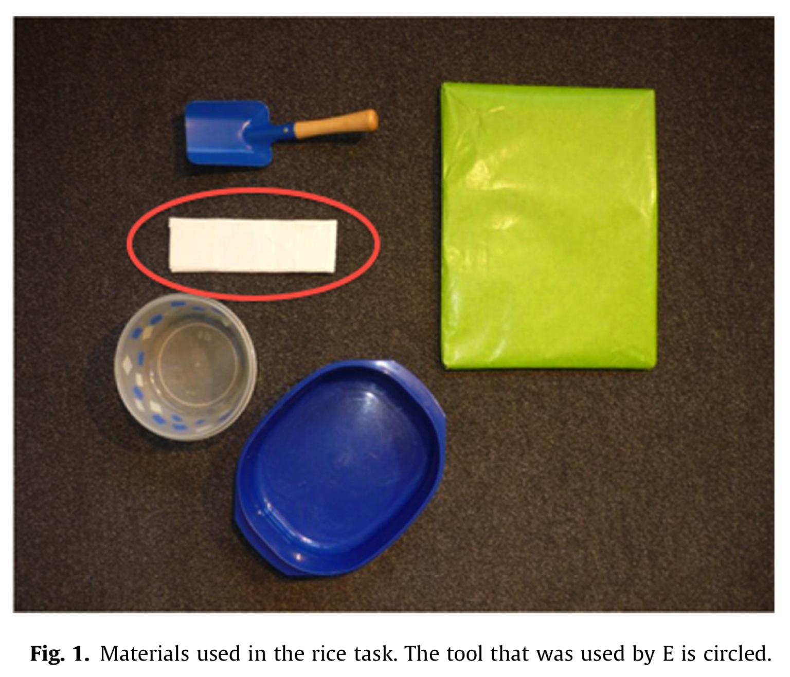
The kids’ task was simple: Try to fill a bucket with as much dry rice as possible. Two kids would be in the room at a time. Kids who completed their turn would swap out for kids who were new to the task, so that there was always 1 kid filling the bucket and 1 kid watching. The kids were given different tools they could potentially use (see their figure 1 below). Some tools were obviously better than others, carrying capacities: Bowl – 817.5g, Bucket – 439.7g, Scoop – 63.9g, Cardboard – 21.5g. In half of the chains, the first child saw an experimenter use the worst tool of the bunch (flimsy cardboard, circled in the figure) and the other half didn’t get a demonstration at all. As always, you can click on the figures to enlarge them.
As the authors said, “A main question of interest was whether children copied [Experimenter]’s and/or the previous child’s choice of tool or whether they innovated by introducing new tools”. In other words, evidence for a ratchet effect would manifest in later generations using more productive tools than the earlier generations. Another interest is whether this innovation differed between conditions- those that had an experimenter demonstrate or not. Not sure why this manipulation is interesting, seeing as the only kids who see the experimenter perform the task are in Generation 1.
Without even going into the stats, I don’t see much evidence that kids are ratcheting. Most chains in the baseline show the following pattern: Generation 1 uses tool X and all subsequent generations use tool X. Two chains manage to break the imitation spell, both switching from scoop+bucket to scoop+bowl. The experimental group shows a similar pattern, where the kids either all copy generation 1 (who copied the experimenter) or one adventurous kid in the chain decides to switch tools and the rest copy him/her. Interestingly, the chains in the experimental group only ever switched from the cardboard to the scoop, effectively going from the worst tool to the second-worst tool. If these kids were trying to score the most rice, wouldn’t it be best to switch to the bucket or the bowl? Weird.
The authors propose that kids in baseline didn’t innovate across generations because they were already performing at a high level in generation 1, so they didn’t have room to grow. Well, the only chains who did actually innovate in baseline started with scoop + bucket (second highest capacity tool) and went to scoop + bowl (highest capacity tool). Further, the chains in the lowest starting position, scoop only, never innovated.
Overall I thought the experiment was cool. Rounding up 80 four year olds is not to be scoffed at. But I don’t agree with their claim that the baseline group was at ceiling and I don’t see much ratcheting in the experimental group (who all start with the worst tool).