My friends did some cool science in 2018

I’ve had a bit of blogger’s block lately (read: the last two years). I have a tendency to write half of a blog post and then scrap it because I don’t think it’s that interesting. Well, my goal this year is to get over it. So to start I decided I want to highlight some of the very cool science my friends did in 2018. Honestly I feel like I don’t do enough to lift up my friends and celebrate their accomplishments, so here are three examples of papers my friends wrote last year that sparked a change in the way I think about one topic or another. I should say, if you aren’t keeping up with these early career researchers, you’re simply missing out on some great science. Happy 2019, everyone!

Improving psychological theory-testing via “systems of orders”

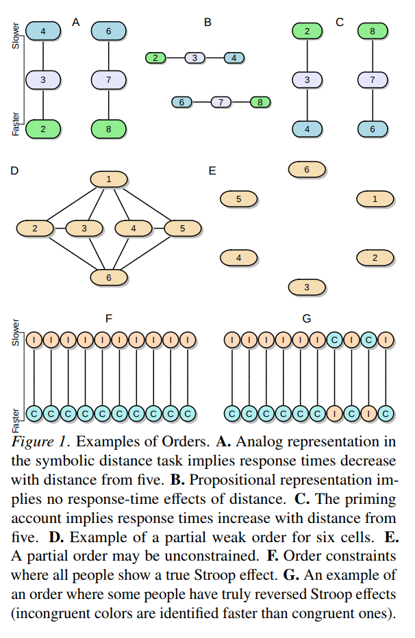
My friend Julia Haaf has been killing it lately (follow her on twitter and check out her google scholar). She just finished her PhD at Missouri and took up a really cool postdoc at the University of Amsterdam, and it feels like every other month she is posting a preprint to some awesome new paper.  One of her papers I’d like to highlight is titled “A note on using systems of orders to capture theoretical constraint in psychological science” (co-authored with Fayette Klaassen and Jeff Rouder), which she presented at APS 2018 in our invited symposium, “Bayesian methods for the pragmatic psychologist.”

This paper really blew me away. One common theme in the ongoing reproducibility debate in psychology is that we need to improve the theory development of our field. The fact is, as psychologists we tend to describe our theories as a set of ordered relationships; e.g., that men respond slower than women in condition A but not condition B. I’m not sure if that will ever change. But when we go to test these directional theories, we usually do something super simple to account for our directional prediction, like a one-sided t-test. Julia and her coauthors describe this process as intellectually inefficient,  because “by positing [a] coarse verbal theory that provides for only modest constraints on the data, we are neither risking nor learning much from the data.” We can do better.

The paper goes on to present a framework that allows us to represent these types of theoretical predictions as sets of explicit order constraints between parameters in a statistical model. Moreover, they demonstrate with nice examples how a Bayesian approach to comparing competing psychological models allows for richer tests of theories in psychology. And come on, just look at this figure. It’s awesome.

haaf_fig

Should we go to the LOO for model selection?

Another person killing it lately is my friend Quentin Gronau (he isn’t on twitter but check out his google scholar page full of interesting work!). Quentin is doing his PhD at the University of Amsterdam, and he blogs at http://www.bayesianspectacles.org from time to time. He and I are at the same stage of our PhD (third year) and we have a lot of overlapping research interests, so I’m always eager to read any paper he writes. One of Quentin’s papers that came out last year that I found quite thought-provoking was titled “Limitations of Bayesian Leave-One-Out Cross-Validation for Model Selection” (co-authored with E.-J. Wagenmakers).

The main idea of this paper is to examine, in the simplest cases possible, the behavior of the Bayesian version of leave-one-out cross-validation (i.e., LOO) when used as a model comparison tool. It turns out that LOO does some weird stuff. For instance, consider comparing models of random guessing vs. informed responding (e.g., H0: θ=.5 vs. H1: θ≠.5) in some binary choice scenario. If we are in a situation where data come in pairs, and if it happens that every pair has 1 success and 1 failure, then we would ideally want our model comparison tool to give more and more evidence for the guessing model as pairs continue to come in. A split pair is, after all, perfectly in line with what the guessing model would predict will happen. If you use LOO for this model comparison, however, the evidence in favor of the guessing model can cap out at a relatively low amount even with observing an infinite number of success-fail pairs.

Also, look at these pretty figures. So damn clean.

The conclusion of this paper was, basically, be careful of LOO if you use it as model comparison tool; if it does weird stuff in super simple cases then how can we be confident it’s doing something sensible in more complex cases? (The paper is more nuanced of course). This paper created quite a stir among some Bayesian circles, and prompted the journal that published it, Computational Brain and Behavior, to invite some very prominent researchers to write commentaries, which I also found quite thought-provoking (find them here, here, and here, and a rejoinder here).  All in all, this paper and the commentaries made me think deeply about model comparison tools and what we should expect from them.

Correlation, causation, and DAGs, oh my!

Another person I want to include in this post is my other friend named Julia: Julia Rohrer (you’ll follow her on twitter and on google scholar if you know what’s good for you). (Both Julias also happen to be German! Julia was apparently the 36th most popular women’s name in Germany in 2017. Wait, Quentin is German too. Wow, the education system over there must be doing something right.)  Julia R. is also in her third year of her PhD –holla!– at the Max Planck Institute for the Life Course in Leipzig, where she is studying personality psychology. ALSO she is simultaneously(!) doing an undergraduate degree in computer science. Last year Julia published what I think is one of the best introductory tutorials out there on causal modeling, titled “Thinking clearly about correlations and causation: Graphical causal models for observational data.”

I think this paper should be required reading for anyone who wants to make causal statements but is limited to collecting observational data. A big challenge when working with observational data is that you can’t rule out confounding factors using randomization like you could in a controlled experiment. This paper outlines a way to model the relationships between variables of interest using what are called “Directed Acyclic Graphs” (i.e., DAGs) to get at the causal inferences we want to make in observational studies. If we create a set of boxes representing variables of interest and arrows that connect them, then if we follow certain rules, voilà, we have ourselves a DAG and maybe a chance at inferring causation. (There’s a bit more to it than just that, of course).

All the figures in this paper are box and arrow causal plots, so I’ll spare you copying them here. Instead I will share some section headers from this paper that I really enjoyed:

  • Confounding: The Bane of Observational Data
  • Learning to Let Go: When Statistical Control Hurts
  • Conclusion: Making Causal Inferences on the Basis of Correlational Data Is Very Hard

What more can I say? Go read these papers right now! You’ll be glad you did!

New revision of How to become a Bayesian in eight easy steps

Quentin, Fabian, Peter, Beth and I recently resubmitted our manuscript titled “How to become a Bayesian in eight easy steps: An annotated reading list” that we initially submitted earlier this year. You can find an updated preprint here. The reviewer comments were pleasantly positive (and they only requested relatively minor changes), so I don’t expect we’ll have another revision. In the revised manuscript we include a little more discussion of the conceptual aspect of Bayes factors (in the summary of source 4), some new discussion on different Bayesian philosophies of how analysis should be done (in the introduction of the “Applied” section) and a few additions to the “Further reading” appendix, among other minor typographical corrections.

This was quite a minor revision. The largest change to the paper by far is our new short discussion on different Bayesian philosophies, which mainly revolve around the (ever-controversial!) issue of hypothesis testing. There is an understandable desire from users of statistics for a unitary set of rules and regulation–a simple list of procedures to follow–where if you do all the right steps you won’t piss off that scrupulous methods guy down the hall from you. Well, as it happens, statistics isn’t like that and you’ll never get that list. Statistics is not just a means to an end, as many substantive researchers tend to think, but an active scientific field itself. Statistics, like any field of study, is a human endeavor that has all sorts of debates and philosophical divides.

Rather than letting these divides turn you off from learning Bayes, I hope they prepare you for the vast analytic viewpoints you will likely encounter as Bayesian analyses become more mainstream. And who knows, maybe you’ll even feel inspired to approach your own substantive problems with a new frame of mind.  Here is an excerpt from our discussion:

Before moving on to our final four highlighted sources, it will be useful if readers consider some differences in perspective among practitioners of Bayesian statistics. The application of Bayesian methods is very much an active field of study, and as such, the literature contains a multitude of deep, important, and diverse viewpoints on how data analysis should be done, similar to the philosophical divides between Neyman–Pearson and Fisher concerning proper application of classical statistics (see Lehmann, 1993). The divide between subjective Bayesians, who elect to use priors informed by theory, and objective Bayesians, who instead prefer “uninformative” or default priors, has already been mentioned throughout the Theoretical sources section above.

.

.
A second division of note exists between Bayesians who see a place for hypothesis testing in science, and those who see statistical inference primarily as a problem of estimation. ….

You’ll have to check out the paper to see how the rest of this discussion goes (see page 10).   🙂

Sunday Bayes: A brief history of Bayesian stats

The following discussion is essentially nontechnical; the aim is only to convey a little introductory “feel” for our outlook, purpose, and terminology, and to alert newcomers to common pitfalls of understanding.

Sometimes, in our perplexity, it has seemed to us that there are two basically different kinds of mentality in statistics; those who see the point of Bayesian inference at once, and need no explanation; and those who never see it, however much explanation is given.

–Jaynes, 1986 (pdf link)

Sunday Bayes

The format of this series is short and simple: Every week I will give a quick summary of a paper while sharing a few excerpts that I like. If you’ve read our eight easy steps paper and you’d like to follow along on this extension, I think a pace of one paper per week is a perfect way to ease yourself into the Bayesian sphere.

Bayesian Methods: General Background

The necessity of reasoning as best we can in situations where our information is incomplete is faced by all of us, every waking hour of our lives. (p. 2)

In order to understand Bayesian methods, I think it is essential to have some basic knowledge of their history. This paper by Jaynes (pdf) is an excellent place to start.

[Herodotus] notes that a decision was wise, even though it led to disastrous consequences, if the evidence at hand indicated it as the best one to make; and that a decision was foolish, even though it led to the happiest possible consequences, if it was unreasonable to expect those consequences. (p. 2)

Jaynes traces the history of Bayesian reasoning all the way back to Herodotus in 500BC. Herodotus could hardly be called a Bayesian, but the above quote captures the essence of Bayesian decision theory: take the action that maximizes your expected gain. It may turn out to be the wrong choice in the end, but if your reasoning that leads to your choice is sound then you took the correct course.

After all, our goal is not omniscience, but only to reason as best we can with whatever incomplete information we have. To demand more than this is to demand the impossible; neither Bernoulli’s procedure nor any other that might be put in its place can get something for nothing. (p. 3)

Much of the foundation for Bayesian inference was actually laid down by James Bernoulli, in his work Ars Conjectandi (“the art of conjecture”) in 1713. Bernoulli was the first to really invent a rational way of specifying a state of incomplete information. He put forth the idea that one can enumerate all “equally possible” cases N, and then count the number of cases for which some event A can occur. Then the probability of A, call it p(A), is just M/N, or the number of cases on which A can occur (M) to the total number of cases (N).

Jaynes gives only a passing mention to Bayes, noting his work “had little if any direct influence on the later development of probability theory” (p. 5). Laplace, Jeffreys, Cox, and Shannon all get a thorough discussion, and there is a lot of interesting material in those sections.

Despite the name, Bayes’ theorem was really formulated by Laplace. By all accounts, we should all be Laplacians right now.

The basic theorem appears today as almost trivially simple; yet it is by far the most important principle underlying scientific inference. (p. 5)

Laplace used Bayes’ theorem to estimate the mass of Saturn, and, by the best estimates when Jaynes was writing, his estimate was correct within .63%. That is very impressive for work done in the 18th century!

This strange history is only one of the reasons why, today [speaking in 1984], we Bayesians need to take the greatest pains to explain our rationale, as I am trying to do here. It is not that it is technically complicated; it is the way we have all been thinking intuitively from childhood. It is just so different from what we were all taught in formal courses on “orthodox” probability theory, which paralyze the mind into an inability to see a distinction between probability and frequency. Students who come to us free of that impediment have no difficulty in understanding our rationale, and are incredulous to anyone that could fail to understand it. (p. 7)

The sections on Laplace, Jeffreys, Cox and Shannon are all very good, but I will skip most of them because I think the most interesting and illuminating section of this paper is “Communication Difficulties” beginning on page 10.

Our background remarks would be incomplete without taking note of a serious disease that has afflicted probability theory for 200 years. There is a long history of confusion and controversy, leading in some cases to a paralytic inability to communicate. (p.10)

Jaynes is concerned in this section with the communication difficulties that Bayesians and frequentists have historically encountered.

[Since the 1930s] there has been a puzzling communication block that has prevented orthodoxians [frequentists] from comprehending Bayesian methods, and Bayesians from comprehending orthodox criticisms of our methods. (p. 10)

On the topic of this disagreement, Jaynes gives a nice quote from L.J. Savage: “there has seldom been such complete disagreement and breakdown of communication since the tower of Babel.” I wrote about one kind of communication breakdown in last week’s Sunday Bayes entry.

So what is the disagreement that Jaynes believes underlies much of the conflict between Bayesians and frequentists?

For decades Bayesians have been accused of “supposing that an unknown parameter is a random variable”; and we have denied hundreds of times with increasing vehemence, that we are making any such assumption. (p. 11)

Jaynes believes the confusion can be made clear by rephrasing the criticism as George Barnard once did.

Barnard complained that Bayesian methods of parameter estimation, which present our conclusions in the form of a posterior distribution, are illogical; for “How could the distribution of a parameter possibly become known from data which were taken with only one value of the parameter actually present?” (p. 11)

Aha, this is a key reformulation! This really illuminates the confusions between frequentists and Bayesians. To show why I’ll give one long quote to finish this Sunday Bayes entry.

Orthodoxians trying to understand Bayesian methods have been caught in a semantic trap by their habitual use of the phrase “distribution of the parameter” when one should have said “distribution of the probability”. Bayesians had supposed this to be merely a figure of speech; i.e., that those who used it did so only out of force of habit, and really knew better. But now it seems that our critics  have been taking that phraseology quite literally all the time.

Therefore, let us belabor still another time what we had previously thought too obvious to mention. In Bayesian parameter estimation, both the prior and posterior distributions represent, not any measurable property of the parameter, but only our own state of knowledge about it. The width of the distribution is not intended to indicate the range of variability of the true values of the parameter, as Barnards terminology had led him to suppose. It indicates the range of values that are consistent with our prior information and data, and which honesty therefore compels us to admit as possible values. What is “distributed” is not the parameter, but the probability. [emphasis added]

Now it appears that, for all these years, those who have seemed immune to all Bayesian explanation have just misunderstood our purpose. All this time, we had thought it clear from our subject-matter context that we are trying to estimate the value that the parameter had at the time the data were taken. [emphasis original] Put more generally, we are trying to draw inferences about what actually did happen in the experiment; not about the things that might have happened but did not. (p. 11)

I think if you really read the section on communication difficulties closely, then you will see that a lot of the conflict between Bayesians and frequentists can be boiled down to deep semantic confusion. We are often just talking past one another, getting ever more frustrated that the other side doesn’t understand our very simple points. Once this is sorted out I think a lot of the problems frequentists see with Bayesian methods will go away.

Sunday Bayes: Optional stopping is no problem for Bayesians

Optional stopping does not affect the interpretation of posterior odds. Even with optional stopping, a researcher can interpret the posterior odds as updated beliefs about hypotheses in light of data.

–Rouder, 2014 (pdf link)

Sunday Bayes

The format of this series is short and simple: Every week I will give a quick summary of a paper while sharing a few excerpts that I like. If you’ve read our eight easy steps paper and you’d like to follow along on this extension, I think a pace of one paper per week is a perfect way to ease yourself into the Bayesian sphere.

Optional stopping: No problem for Bayesians

Bayesian analysts use probability to express a degree of belief. For a flipped coin, a probability of 3/4 means that the analyst believes it is three times more likely that the coin will land heads than tails. Such a conceptualization is very convenient in science, where researchers hold beliefs about the plausibility of theories, hypotheses, and models that may be updated as new data become available. (p. 302)

It is becoming increasingly common to evaluate statistical procedures by way of simulation. Instead of doing formal analyses, we can use flexible simulations to tune many different parameters and immediately see the effect it has on the behavior of a procedure.

Simulation results have a tangible, experimental feel; moreover, if something is true mathematically, we should be able to see it in simulation as well. (p. 303)

But this brings with it a danger that the simulations performed might be doing the wrong thing, and unless we have a good grasp of the theoretical background of what is being simulated we can easily be misled. In this paper, Rouder (pdf) shows that common intuitions we have for evaluating simulations of frequentist statistics often do not translate to simulations of Bayesian statistics.

The critical element addressed here is whether optional stopping is problematic for Bayesians. My  argument is that both sets of authors use the wrong criteria or lens to draw their conclusions. They evaluate and interpret Bayesian statistics as if they were frequentist statistics. The more germane question is whether Bayesian statistics are interpretable as Bayesian statistics even if data are collected under optional stopping. (p. 302)

When we evaluate a frequentist procedure via simulation, it is common to set a parameter to a certain value and evaluate the number of times certain outcomes occur. For example, we can set the difference between two group means to zero, simulate a bunch of p values, and see how many fall below .05. Then we can set the difference to some nonzero number, simulate a bunch of p values, and again see how many are below .05. The first gives you the type-1 error rate for the procedure, and the second gives you the statistical power. This is appropriate for frequentist procedures because the probabilities calculated are always conditional on one or the other hypothesis being true.

One might be tempted to evaluate Bayes factors in the same way; that is, set the difference between two groups to zero and see how many BFs are above some threshold, and then set the difference to something nonzero and see how many BFs are again above some threshold.

The critical error … is studying Bayesian updating conditional on some hypothetical truth rather than conditional on data. This error is easy to make because it is what we have been taught and grown familiar with in our frequentist training. (p. 308)

Evaluating simulations of Bayes factors in this way is incorrect. Bayes factors (and posterior odds) are conditional on only the data observed. In other words, the appropriate evaluation is: “Given that I have observed this data (i.e., BF = x), what is the probability the BF was generated by H1 vs H0?”

Rouder visualizes this as follows. Flip a coin to choose the true hypothesis, then simulate a Bayes factor, and repeat these two steps many many times. At the end of the simulation, whenever BF=x is observed, check and see how many of these came from one model vs the other. The simulation shows that in this scenario if we look at all the times BF=3 is observed, there will be 3 BFs from the true model to every 1 BF from the false model. Since the prior odds are 1 to 1, the posterior odds equals the Bayes factor.

Screenshot 2016-03-06 12.33.59

You can see in the figure above (taken from Rouder’s figure 2), the distribution of Bayes factors observed when the null is true (purple, projected downwards) vs when the alternative is true (pink, projected upwards). Remember, the true hypothesis was chosen by coin flip. You can clearly see that when a BF of 3 to 1 in favor of the null is observed, the purple column is three times bigger than the pink column (shown with the arrows).

Below (taken from Rouder’s figure 2) you see what happens when one employs optional stopping (e.g., flip a coin to pick underlying true model, then sample until BF favors one model to another by at least 10 or you reach a maximum n). The distribution of Bayes factors generated by each model becomes highly skewed, which is often taken as evidence that conclusions drawn from Bayes factors depend on the stopping rule. The incorrect interpretation would be: Given the null is true, the number of times I find BF=x in favor of the alternative (i.e., in favor of the wrong model) has gone up, therefore the BF is sensitive to optional stopping. This is incorrect because it conditions on one model being true and checks the number of times a BF is observed, rather than conditioning on the observed BF and checking how often it came from H0 vs. H1.

Look again at what matters: What is the ratio of observed BFs that come from H1 vs. H0 for a given BF? No matter what stopping rule is used, the answer is always the same: If the true hypothesis is chosen by a coin flip, and a BF of 10 in favor of the alternative is observed, there will be 10 times as many observed BFs in the alternative column (pink) than in the null column (purple).

Screenshot 2016-03-06 12.40.31

In Rouder’s simulations he always used prior odds of 1 to 1, because then the posterior odds equal the Bayes factor. If one were to change the prior odds then the Bayes factor would no longer equal the posterior odds, and the shape of the distribution would again change; but importantly, while the absolute number of Bayes factors that end up in each bin would change, but the ratios of each pink column to purple column would not. No matter what stopping rule you use, the conclusions we draw from Bayes factors and posterior odds are unaffected by the stopping rule.

Feel free to employ any stopping rule you wish.

This result was recently shown again by Deng, Lu, and Chen in a paper posted to arXiv (pdf link) using similar simulations, and they go further in that they prove the theorem.

A few choice quotes

Page 308:

Optional-stopping protocols may be hybrids where sampling occurs until the Bayes factor reaches a certain level or a certain number of samples is reached. Such an approach strikes me as justifiable and reasonable, perhaps with the caveat that such protocols be made explicit before data collection. The benefit of this approach is that more resources may be devoted to more ambiguous experiments than to clear ones.

Page 308:

The critical error … is studying Bayesian updating conditional on some hypothetical truth rather than conditional on data. This error is easy to make because it iswhat we have been taught and grown familiar with in our frequentist training. In my opinion, the key to understanding Bayesian analysis is to focus on the degree of belief for considered models, which need not and should not be calibrated relative to some hypothetical truth.

Page 306-307:

When we update relative beliefs about two models, we make an implicit assumption that they are worthy of our consideration. Under this assumption, the beliefs may be updated regardless of the stopping rule. In this case, the models are dramatically wrong, so much so that the posterior odds contain no useful information whatsoever. Perhaps the more important insight is not that optional stopping is undesirable, but that the meaningfulness of posterior odds is a function of the usefulness of the models being compared.

Sunday Bayes: Testing precise hypotheses

First and foremost, when testing precise hypotheses, formal use of P-values should be abandoned. Almost anything will give a better indication of the evidence provided by the data against Ho.

–Berger & Delampady, 1987 (pdf link)

Sunday Bayes series intro:

After the great response to the eight easy steps paper we posted, I started a recurring series, where each week I highlight one of the papers that we included in the appendix of the paper. The format is short and simple: I will give a quick summary of the paper while sharing a few excerpts that I like. If you’ve read our eight easy steps paper and you’d like to follow along on this extension, I think a pace of one paper per week is a perfect way to ease yourself into the Bayesian sphere. At the end of the post I will list a few suggestions for the next entry, so vote in the comments or on twitter (@alxetz) for which one you’d like next. This paper was voted to be the next in the series.

(I changed the series name to Sunday Bayes, since I’ll be posting these on every Sunday.)

Testing precise hypotheses

This would indicate that say, claiming that a P-value of .05 is significant evidence against a precise hypothesis is sheer folly; the actual Bayes factor may well be near 1, and the posterior probability of Ho near 1/2 (p. 326)

Berger and Delampady (pdf link) review the background and standard practice for testing point null hypotheses (i.e., “precise hypotheses”). The paper came out nearly 30 years ago, so some parts of the discussion may not be as relevant these days, but it’s still a good paper.

They start by reviewing the basic measures of evidence — p-values, Bayes factors, posterior probabilities — before turning to an example. Rereading it, I remember why we gave this paper one of the highest difficulty ratings in the eight steps paper. There is a lot of technical discussion in this paper, but luckily I think most of the technical bits can be skipped in lieu of reading their commentary.

One of the main points of this paper is to investigate precisely when it is appropriate to approximate a small interval null hypothesis by using a point null hypothesis. They conclude, that most of the time, the error of approximation for Bayes factors will be small (<10%),

these numbers suggest that the point null approximation to Ho will be reasonable so long as [the width of the null interval] is one-half a [standard error] in width or smaller. (p. 322)

A secondary point of this paper is to refute the claim that classical answers will typically agree with some “objective” Bayesian analyses. Their conclusion is that such a claim

is simply not the case in the testing of precise hypotheses. This is indicated in Table 1 where, for instance, P(Ho | x) [NB: the posterior probability of the null] is from 5 to 50 times larger than the P-value. (p. 318)

They also review some lower bounds on the amount of Bayesian evidence that corresponds to significant p-values. They sum up their results thusly,

The message is simple: common interpretation of P-values, in terms of evidence against precise [null] hypotheses, are faulty (p. 323)

and

the weighted likelihood of H1 is at most [2.5] times that of Ho. A likelihood ratio [NB: Bayes factor] of [2.5] is not particularly strong evidence, particularly when it is [an upper] bound. However, it is customary in practice to view [p] = .05 as strong evidence against Ho. A P-value of [p] = .01, often considered very strong evidence against Ho, corresponds to [BF] = .1227, indicating that H1 is at most 8 times as likely as Ho. The message is simple: common interpretation of P-values, in terms of evidence against precise [null] hypotheses, are faulty (p. 323)

A few choice quotes

Page 319:

[A common opinion is that if] θ0 [NB: a point null] is not in [a confidence interval] it can be rejected, and looking at the set will provide a good indication as to the actual magnitude of the difference between θ and θ0. This opinion is wrong, because it ignores the supposed special nature of θo. A point can be outside a 95% confidence set, yet not be so strongly contraindicated by the data. Only by calculating a Bayes factor … can one judge how well the data supports a distinguished point θ0.

Page 327:

Of course, every statistician must judge for himself or herself how often precise hypotheses actually occur in practice. At the very least, however, we would argue that all types of tests should be able to be properly analyzed by statistics

Page 327 (emphasis original, since that text is a subheading):

[It is commonly argued that] The P-Value Is Just a Data Summary, Which We Can Learn To Properly Calibrate … One can argue that, through experience, one can learn how to interpret P-values. … But if the interpretation depends on Ho, the sample size, the density and the stopping rule, all in crucial ways, it becomes ridiculous to argue that we can intuitively learn to properly calibrate P-values.

page 328:

we would urge reporting both the Bayes factor, B, against [H0] and a confidence or credible region, C. The Bayes factor communicates the evidence in the data against [H0], and C indicates the magnitude of the possible discrepancy.

Page 328:

Without explicit alternatives, however, no Bayes factor or posterior probability could be calculated. Thus, the argument goes, one has no recourse but to use the P-value. A number of Bayesian responses to this argument have been raised … here we concentrate on responding in terms of the discussion in this paper. If, indeed, it is the case that P-values for precise hypotheses essentially always drastically overstate the actual evidence against Ho when the alternatives are known, how can one argue that no problem exists when the alternatives are not known?


Vote for the next entry:

  1. Edwards, Lindman, and Savage (1963) — Bayesian Statistical Inference for Psychological Research (pdf)
  2. Rouder (2014) — Optional Stopping: No Problem for Bayesians (pdf)
  3. Gallistel (2009) — The Importance of Proving the Null (pdf)
  4. Lindley (2000) — The philosophy of statistics (pdf)