[This post has been updated and turned into a paper to be published in AMPPS]
Much of the discussion in psychology surrounding Bayesian inference focuses on priors. Should we embrace priors, or should we be skeptical? When are Bayesian methods sensitive to specification of the prior, and when do the data effectively overwhelm it? Should we use context specific prior distributions or should we use general defaults? These are all great questions and great discussions to be having.
One thing that often gets left out of the discussion is the importance of the likelihood. The likelihood is the workhorse of Bayesian inference. In order to understand Bayesian parameter estimation you need to understand the likelihood. In order to understand Bayesian model comparison (Bayes factors) you need to understand the likelihood and likelihood ratios.
What is likelihood?
Likelihood is a funny concept. It’s not a probability, but it is proportional to a probability. The likelihood of a hypothesis (H) given some data (D) is proportional to the probability of obtaining D given that H is true, multiplied by an arbitrary positive constant (K). In other words, L(H|D) = K · P(D|H). Since a likelihood isn’t actually a probability it doesn’t obey various rules of probability. For example, likelihood need not sum to 1.
A critical difference between probability and likelihood is in the interpretation of what is fixed and what can vary. In the case of a conditional probability, P(D|H), the hypothesis is fixed and the data are free to vary. Likelihood, however, is the opposite. The likelihood of a hypothesis, L(H|D), conditions on the data as if they are fixed while allowing the hypotheses to vary.
The distinction is subtle, so I’ll say it again. For conditional probability, the hypothesis is treated as a given and the data are free to vary. For likelihood, the data are a given and the hypotheses vary.
The Likelihood Axiom
Edwards (1992, p. 30) defines the Likelihood Axiom as a natural combination of the Law of Likelihood and the Likelihood Principle.
The Law of Likelihood states that “within the framework of a statistical model, a particular set of data supports one statistical hypothesis better than another if the likelihood of the first hypothesis, on the data, exceeds the likelihood of the second hypothesis” (Emphasis original. Edwards, 1992, p. 30).
In other words, there is evidence for H1 vis-a-vis H2 if and only if the probability of the data under H1 is greater than the probability of the data under H2. That is, D is evidence for H1 over H2 if P(D|H1) > P(D|H2). If these two probabilities are equivalent, then there is no evidence for either hypothesis over the other. Furthermore, the strength of the statistical evidence for H1 over H2 is quantified by the ratio of their likelihoods, L(H1|D)/L(H2|D) (which again is proportional to P(D|H1)/P(D|H2) up to an arbitrary constant that cancels out).
The Likelihood Principle states that the likelihood function contains all of the information relevant to the evaluation of statistical evidence. Other facets of the data that do not factor into the likelihood function are irrelevant to the evaluation of the strength of the statistical evidence (Edwards, 1992, p. 30; Royall, 1997, p. 22). They can be meaningful for planning studies or for decision analysis, but they are separate from the strength of the statistical evidence.
Likelihoods are meaningless in isolation
Unlike a probability, a likelihood has no real meaning per se due to the arbitrary constant. Only by comparing likelihoods do they become interpretable, because the constant in each likelihood cancels the other one out. The easiest way to explain this aspect of likelihood is to use the binomial distribution as an example.
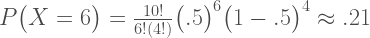
Suppose I flip a coin 10 times and it comes up 6 heads and 4 tails. If the coin were fair, p(heads) = .5, the probability of this occurrence is defined by the binomial distribution:

where x is the number of heads obtained, n is the total number of flips, p is the probability of heads, and

Substituting in our values we get
If the coin were a trick coin, so that p(heads) = .75, the probability of 6 heads in 10 tosses is:

To quantify the statistical evidence for the first hypothesis against the second, we simply divide one probability by the other. This ratio tells us everything we need to know about the support the data lends to one hypothesis vis-a-vis the other. In the case of 6 heads in 10 tosses, the likelihood ratio (LR) for a fair coin vs our trick coin is:

Translation: The data are 1.4 times as probable under a fair coin hypothesis than under this particular trick coin hypothesis. Notice how the first terms in each of the equations above, i.e., 
Same data. Same constant. Cancel out.
The first term in the equations above,
If we leave out the first term in the above calculations, our numerator is L(.5) = 0.0009765625 and our denominator is L(.75) ≈ 0.0006952286. Using these values to form the likelihood ratio we get: 0.0009765625/0.0006952286 ≈ 1.4, as we should since the other terms simply cancelled out before.
Again I want to reiterate that the value of a single likelihood is meaningless in isolation; only in comparing likelihoods do we find meaning.
Looking at likelihoods
Likelihoods may seem overly restrictive at first. We can only compare 2 simple statistical hypotheses in a single likelihood ratio. But what if we are interested in comparing many more hypotheses at once? What if we want to compare all possible hypotheses at once?
In that case we can plot the likelihood function for our data, and this lets us ‘see’ the evidence in its entirety. By plotting the entire likelihood function we compare all possible hypotheses simultaneously. The Likelihood Principle tells us that the likelihood function encompasses all statistical evidence that our data can provide, so we should always plot this function along side our reported likelihood ratios.
Following the wisdom of Birnbaum (1962), “the “evidential meaning” of experimental results is characterized fully by the likelihood function” (as cited in Royall, 1997, p.25). So let’s look at some examples. The R script at the end of this post can be used to reproduce these plots, or you can use it to make your own plots. Play around with it and see how the functions change for different number of heads, total flips, and hypotheses of interest. See the instructions in the script for details.
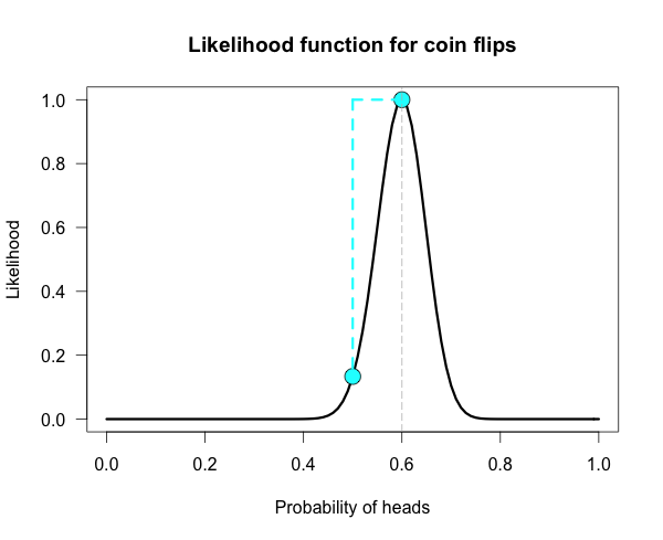
Below is the likelihood function for 6 heads in 10 tosses. I’ve marked our two hypotheses from before on the likelihood curve with blue dots. Since the likelihood function is meaningful only up to an arbitrary constant, the graph is scaled by convention so that the best supported value (i.e., the maximum) corresponds to a likelihood of 1.

The vertical dotted line marks the hypothesis best supported by the data. The likelihood ratio of any two hypotheses is simply the ratio of their heights on this curve. We can see from the plot that the fair coin has a higher likelihood than our trick coin.
How does the curve change if instead of 6 heads out of 10 tosses, we tossed 100 times and obtained 60 heads?

Our curve gets much narrower! How did the strength of evidence change for the fair coin vs the trick coin? The new likelihood ratio is L(.5)/L(.75) ≈ 29.9. Much stronger evidence!(footnote) However, due to the narrowing, neither of these hypothesized values are very high up on the curve anymore. It might be more informative to compare each of our hypotheses against the best supported hypothesis. This gives us two likelihood ratios: L(.6)/L(.5) ≈ 7.5 and L(.6)/L(.75) ≈ 224.
Here is one more curve, for when we obtain 300 heads in 500 coin flips.

Notice that both of our hypotheses look to be very near the minimum of the graph. Yet their likelihood ratio is much stronger than before. For this data the likelihood ratio L(.5)/L(.75) is nearly 24 million! The inherent relativity of evidence is made clear here: The fair coin was supported when compared to one particular trick coin. But this should not be interpreted as absolute evidence for the fair coin, because the likelihood ratio for the maximally supported hypothesis vs the fair coin, L(.6)/L(.5), is nearly 24 thousand!
We need to be careful not to make blanket statements about absolute support, such as claiming that the maximum is “strongly supported by the data”. Always ask, “Compared to what?” The best supported hypothesis will be only be weakly supported vs any hypothesis just before or just after it on the x-axis. For example, L(.6)/L(.61) ≈ 1.1, which is barely any support one way or the other. It cannot be said enough that evidence for a hypothesis must be evaluated in consideration with a specific alternative.
Connecting likelihood ratios to Bayes factors
Bayes factors are simple extensions of likelihood ratios. A Bayes factor is a weighted average likelihood ratio based on the prior distribution specified for the hypotheses. (When the hypotheses are simple point hypotheses, the Bayes factor is equivalent to the likelihood ratio.) The likelihood ratio is evaluated at each point of the prior distribution and weighted by the probability we assign that value. If the prior distribution assigns the majority of its probability to values far away from the observed data, then the average likelihood for that hypothesis is lower than one that assigns probability closer to the observed data. In other words, you get a Bayes boost if you make more accurate predictions. Bayes factors are extremely valuable, and in a future post I will tackle the hard problem of assigning priors and evaluating weighted likelihoods.
I hope you come away from this post with a greater knowledge of, and appreciation for, likelihoods. Play around with the R code and you can get a feel for how the likelihood functions change for different data and different hypotheses of interest.
(footnote) Obtaining 60 heads in 100 tosses is equivalent to obtaining 6 heads in 10 tosses 10 separate times. To obtain this new likelihood ratio we can simply multiply our ratios together. That is, raise the first ratio to the power of 10; 1.4^10 ≈ 28.9, which is just slightly off from the correct value of 29.9 due to rounding.
R Code
| ## Plots the likelihood function for the data obtained | |
| ## h = number of successes (heads), n = number of trials (flips), | |
| ## p1 = prob of success (head) on H1, p2 = prob of success (head) on H2 | |
| ## Returns the likelihood ratio for p1 over p2. The default values are the ones used in the blog post | |
| LR <- function(h,n,p1=.5,p2=.75){ | |
| L1 <- dbinom(h,n,p1)/dbinom(h,n,h/n) ## Likelihood for p1, standardized vs the MLE | |
| L2 <- dbinom(h,n,p2)/dbinom(h,n,h/n) ## Likelihood for p2, standardized vs the MLE | |
| Ratio <- dbinom(h,n,p1)/dbinom(h,n,p2) ## Likelihood ratio for p1 vs p2 | |
| curve((dbinom(h,n,x)/max(dbinom(h,n,x))), xlim = c(0,1), ylab = "Likelihood",xlab = "Probability of heads",las=1, | |
| main = "Likelihood function for coin flips", lwd = 3) | |
| points(p1, L1, cex = 2, pch = 21, bg = "cyan") | |
| points(p2, L2, cex = 2, pch = 21, bg = "cyan") | |
| lines(c(p1, p2), c(L1, L1), lwd = 3, lty = 2, col = "cyan") | |
| lines(c(p2, p2), c(L1, L2), lwd = 3, lty = 2, col = "cyan") | |
| abline(v = h/n, lty = 5, lwd = 1, col = "grey73") | |
| return(Ratio) ## Returns the likelihood ratio for p1 vs p2 | |
| } |
References
Birnbaum, A. (1962). On the foundations of statistical inference. Journal of the American Statistical Association, 57(298), 269-306.
Edwards, A. W. (1992). Likelihood, expanded ed. Johns Hopkins University Press.
Royall, R. (1997). Statistical evidence: A likelihood paradigm (Vol. 71). CRC press.

Dear Alex Etz,
thank you for this informative post. I think it provides a clear basic introduction to the logic of Bayes-Factors.
The likelihood function plots are particularly informative. What should a researcher conclude from the likelihood plot for 300 heads with 500 coin flips is particularly informative because it has the largest sample size. A simple visual inspections shows that there is very little empirical support for either one of the two a priori hypothesis (p = .50 & p = .75). Moreover, BF comparisons of the a priori hypothesis with the observed data favor the observed data (.60) over the a priori hypothesis .50 and .75. In short the data favor .60 over the a priori hypothesis .50, which is the null-hypothesis that the odds for heads and tail are equal (.50 – .50 = 0).
A traditional significance test would have shown that the probability of obtaining 300 out of 500 heads for a fair coin (a priori hypothesis .50) is p < .00001. It is therefore very safe to reject the null-hypothesis and to conclude that the coin is not fair.
The standard Bayesian argument against the use of p-values in this scenario is that we do not know how the 500 trials were conducted and that the researcher may have capitalized on chance by stopping whenever the result was significant. But how would be explain that the p-value is well below any significance criterion like p < .05. This is inconsistent with optional stopping. Moreover, you can run simulations to see how often optional stopping would produce a result like 300 out of 500 heads. Optional stopping simply does not have the power to produce such a strong effect.
The BF makes things murky because it also tests an alternative hypothesis, p = .75. Where does this hypothesis come from. Why not p = .55, .60, or .95 as alternative. The arbitrary choice of an alternative is the key weakness of BF. They are internally consistent, but they do not tell us what most researchers want to know. Is the coin fair? Not, is the coin more likely to be fair than to be biased by a certain amount.
Take quality control in a casino as an example. The casino makes money from a fair roulette table (equal odds for red and black, take all the money for green). One casino uses frequentists statistics to test whether a table is fair. After 500 games they discover that red occurred 300 times. They remove the table because savy gamblers started capitalizing on the good odds for red on this table. The Bayesian casino tests p = .50 against p = .75. As the actual odds are .60, the BF favors the hypothesis that the table is fair over the hypothesis that the table is biased (increased odds of 50:50 to 75:25) and they keep the table in play. They bayesian casino loses money because frequentists gamblers have figured out that the table gives them better odds of winning.
Frequentists win when Bayesians compute BF with bad priors. So, the trick is to have good priors. Welcome to the world of unknowns. Bayesian statistics is a religion that gives a false promise of certainty to believers in a world of uncertainty.
Sincerely, Dr. R
Hi Dr. R,
Thank you for reading, I really appreciate your kind compliments 🙂 Here is my long-winded reply.
>>”The standard Bayesian argument against the use of p-values in this scenario is that we do not know how the 500 trials were conducted and that the researcher may have capitalized on chance by stopping whenever the result was significant. ”
My argument is simpler than that. p values depend on stopping rules. If you don’t know the stopping rule, you don’t know the real value of p. If you don’t preregister the study, there is no way to know the real value of p. The argument is not that the researchers are necessarily wrong (although sometimes they almost surely are), but instead that their arguments are not justified by the evidence they provide.
A second argument is that the law of improbability (obtain low p, reject the null) is fallacious. That something is rare under a hypothesis is not logically evidence against the hypothesis. We could go into that but it would be a lot of typing. See Royall’s book, chapter 3 for more. Let me know if you want to hash it out and I’ll be happy to talk about it with you.
The point of this post is not to argue about which statistics we should be using, but to explain what likelihoods are and why they are valuable. If you don’t think they add value to your analysis, don’t use them. I am happy to give you the information about what they are and how they work and let you decide for yourself what you should do. If you want to know more about them and their properties I am happy to be a resource as best I can. But you should know that Neyman-Pearson theory (and power) is based on a variant of likelihood.
>>”The BF makes things murky because it also tests an alternative hypothesis, p = .75.”
I can’t possibly fathom how you are against testing or even proposing alternative hypotheses, given that you are so big on power. Do you see the irony here? Power is only controlled for a process, in principle and practice, when you have well-defined, predetermined hypotheses that form rejection regions that exhaust the sample space.
I can’t stress this enough: The entire point of power as a concept is that there are alternative hypotheses being tested.
>>“Where does this hypothesis come from. Why not p = .55, .60, or .95 as alternative. The arbitrary choice of an alternative is the key weakness of BF. ”
The alternative can come from literally anywhere. It can even come from the actual data and it does not change the likelihood ratios. Where we get our hypotheses from does not change their relative support. Again, I am so confused about why you are against defining alternative hypotheses. If you could clarify for me I would actually really appreciate it. Either a comment here or a post on your blog explaining it would be welcome.
The alternative hypothesis in this post was an arbitrary example, because it was used for illustrative purposes to help people understand the concept. If there was a theoretically motivated reason to think about different values of course researchers could do that. You ask why not choose .55, or .60, or .95. The point of plotting the entire likelihood function is that these choices become irrelevant. You see all possible comparisons at once. The fact that going into the study you were initially interested in .5 vs .75, or anything else, is irrelevant once the data are in. Just look at the curve and it tells you everything you need to know. The same is true if you are doing Bayesian posterior estimation. Plot the full curve and just look at it.
>>”Take quality control in a casino as an example.”
Your casino example is misguided. You are conflating inference with decision theory. To make decisions you must have an alternative hypothesis, otherwise you cannot determine the utility of taking one action over another based on your inference. If they are trying to make decisions about whether they should keep the tables on the floor they need to determine the costs/benefits of it being fair or a little unfair or a lot unfair. If it costs more to replace all of the tables on their floor than the money they lose from slightly unfair tables being gamed by a few people, then it makes sense to keep the tables they have even if they are not 100% fair. That is just one example, I’m sure we could brainstorm 100 different utility functions for this based on different aspects of the problem.
Dear Alex,
1. You overestimate the effect of optional stopping on p-values. Optional stopping can create a bias, but not to the extent that p-values cannot be interpreted when the stopping rule is unknown. You can run some simulations or check out Sanborn and Hills (2014).
Of course, why not just use Bayes-Factor that are immune to stopping rules? The answer is that you have to specify an a priori alternative to the null-hypothesis. That seems risky when you do not know anything about a research domain and you want to see whether there is an effect without knowing how strong the effect is.
Power analysis is not the same as testing two alternative hypotheses. The main purpose of a priori power analysis is to determine sample size to have a good chance to reject the null-hypothesis is false. The alternative is still d > 0, but it makes only sense to test this hypothesis if the alternative has a fighting chance.
Finally, your example with .5 and .75 and a coin that actually has a bias of .6, is a good example, where the alternative was chosen too high. As the difference between .5 and .6 is smaller than .6 and .75, BF will decide in favor of .5. IF you had contrasted .5 with .65, BF would have favored the alternative hypothesis over the null-hypothesis.
In short, there is no free lunch and Bayesian statistic is not a magical tool. To win immunity against optional stopping you have to pay a price that you can only test the null-hypothesis against an alternative. When both hypotheses are false, optional stopping with BF can lead to wrong conclusions.
Further reading:
The Frequentist Implications of Optional Stopping on Bayesian Hypothesis Tests
Adam N. Sanborn Thomas T. Hills
http://link.springer.com/article/10.3758%2Fs13423-013-0518-9
Your definition of power is not the one I learned. Could you point me to a reference that I can read to try to understand the rationale?
http://www.amazon.com/Statistical-Analysis-Behavioral-Sciences-Edition/dp/0805802835
The main point is that SST (statistical significance testing) never concludes in favor of the point-null-hypothesis. If a study had insufficient power, it is likely to produce a type-II error (a failure to reject the false null-hypothesis). This is sometimes falsely interpreted or reported as evidence that “there is no effect”, but the correct inference is that the study had insufficient evidence to determine whether there is an effect or no effect.
In contrast, Bayesian hypothesis testing (BHT) explicitly tests whether the null-hypothesis is true(er than an alternative) and BF are interpreted as evidence in favor of the null (as opposed to some alternative). This is radically different because this approach can create false positives for the null-hypothesis (the BF factor strongly favors the null [over an alternative], but the null is false.
Your own example would be such a false positive because the BF favors p = .5 (over p = .75) when p = .5 (there is no bias) is false and p = .6 (there is bias) is true.
The criticism of BF is that it will often make false positive errors in favor of the null, when the true effect size is small and the alternative is larger (more than two times the true effect size). This does not change when you make the alternative a distribution rather than a point estimate. As you point out the distribution is essentially a weighted average of point estimates, so if the weighted average of point estimates is twice as large as the true effect size, BF will make a false positive in favor of the null.
You may say that this is not a problem because in the long run the posteriori distribution will spike over the true effect size, but that is simply saying that in the limit the sample mean approaches the population mean. In actual empirical studies data collection will often end before the data provide a good estimate of the population effect size.
This is where optional stopping comes in. BHT is often sold as superior because it is internally coherent when you test after each participants. However, optional stopping introduces a decision process. When do I stop data collection. The problem is that the the final result depends on the decision criterion and that BF 10 in favor of a small effect size is rarely reached in small samples. On the other hand, BF 10 in favor of null can be achieved with small effect sizes quite easily if the alternative specifies a strong effect size. In this scenario optional stopping with BF will have many false negatives (failure to detect a small effect) AND many false positives (falsely favoring the null-hypothesis when it is not true). You can try it out with your own simulations and a between -subject design, d = .2, and sampling from 20 to 50 participants in each condition. How often does BHT correctly confirm the presence of a small effect and how often does it falsely decide in favor of the null-hypothesis?
In short, once you use optional stopping, you have to think about the decision rule that terminates data collection. This may not be a problem for BHT in general, but it is a problem for BHT with optional stopping.
Thanks for the fun post, Alex. I especially like the point near the end about the natural relationship between likelihood tests and Bayes factors — I hadn’t really considered the Bayes factor as a “weighted” likelihood test before!
I wanted to chip in and see if I could clarify a few points for Dr. R. He says:
“The main purpose of a priori power analysis is to determine sample size to have a good chance to reject the null-hypothesis is false. The alternative is still d > 0, but it makes only sense to test this hypothesis if the alternative has a fighting chance.”
A priori power is contingent on three numbers: alpha threshold, sample size, and a hypothetical true effect size. When you’re firing up G*Power, you’ll notice your power depends a lot on what you think the effect size might be: You could have 95% power to detect d = 1.0, but only 25% power to detect d = 0.3.
So the point that I think Alex is trying to make, then, is that our concept of whether a study is “properly powered” or “underpowered” depends heavily on what we think the true effect size might be. In other words, power depends on our alternative hypothesis. If H1 is d = 1.0, we have good power; if H1 is d = 0.3, we have poor power.
Which of these options is right? Well, we’ll never know for sure. We’ll have to use our own good judgment. This is what it means to place priors: Your interpretation of the experiment as well-powered or insufficiently-powered depends on what your prior on the effect size is.
My second point (that Alex seems to be foreshadowing here) is that Bayesians don’t have to pick a single point-value for the alternative hypothesis. Likelihoodists have to for their ratio tests (as in the blog post above), and frequentists have to for a priori power calculation.
When choosing those point-values, you might be worried that you’re choosing the wrong point. Is the study well-powered (d = 1.0, power = 95%) or underpowered (d = 0.3, power = 25%)?
Bayesians don’t have to select a single point if they don’t want to. Instead, they can choose a distribution of values. We might say d ~ Uniform(0, 1) or d ~ Normal(.5, 1). By spreading the probability around a little bit, I think the results can be –more– robust than they might be when having to select a single value.
So again, I just wanted to try to point out that a priori power analysis does require formulating an alternative hypothesis. Since we believe well-powered tests and don’t believe underpowered tests, power analysis does a lot to influence whether we believe a significant result or not. So your prior belief in a particular effect size guides your judgments are surely as any Bayesian’s prior does.
– Joe
Power analysis does require an assumption about the population effect size to plan a study.
However, the actual tests only tests H0 (d = 0) against an unspecified range of possible effect sizes (d > 0).
A significant result does not confirm that the effect size used in the power analysis is the true effect size. It only provides evidence that the effect size is greater than 0.
You may enter d = .8 in a power analysis and run a study with 80% power. A significant result still only means the effect is greater than 0. It does not mean you showed evidence for d = .8.
This is the key difference to Bayesian Hypothesis testing, where you test d = 0 against d = .8 (or a distribution) and then conclude in favor of one of these hypotheses.
I see. So are you as convinced by N=20, p = .049 as you are by N = 2,000, p < .001? Both yield the same significant test result, and you seem to imply in the above comment that considerations of a priori power do not influence interpretation of the test result.
In practice, I think that you are indeed concerned about significant test results that are "underpowered", as the word comes up quite frequently in your blog posts. I do not think you believe in N = 20, p = .049 like you do N = 2000, p < .001. But again, whether we consider a significance test to be well-powered or underpowered depends substantially on what we think a likely effect size might be: our prior expectation.
Dear Joe,
there is an interpretation of significance testing that all p-values below .05 are equal. However, just as there is no real difference between p = .04 and p = .06, there is a real difference between .049 and .001.
Even Bayesians cannot publish an article without drawing some conclusions, which means to draw some inferences from a study that goes beyond the sample. BF > 3, favors hypothesis, BF > 10 strong support for hypothesis, etc.
equate p with BF and you have a continuous measure of evidence, so there is just no difference between significance testing and Bayesian hypothesis testing that in a world of uncertainty you can quantify risk of being wrong, but you can never be certain.
Underpowered studies are a problem for two reasons. First, honest reporting of non-significant results tells us very little. The effect size could have been anywhere between 0 and .8 before the study and after the study so why do a study? Second, a significant result would be informative if we could be sure that all data were reported. As you know, this is not the case. The R-Index is a tool that can examine whether a set of studies is credible. If 100 studies would show 30 significant results and 70 non-significant results and average observed power is 30%, I would conclude that the null-hypothesis is false. I would also point out that this conclusion could have been reached much faster with a few high powered studies that would have consistently shown significant results (say 5 studies with 80% power and one non-significant result).
BHT and SST are not so different when it comes to demonstrating effects that are actually present. The key difference is how BHT and SST deal with evidence where the null-hypothesis may be true. There is a temptation to use BHT to prove the null-hypothesis to be true, but I think this is impossible. It is possible to demonstrate that an effect cannot be larger than a particular value (say d < .01), but this can be done with BHT and SST and it requires a lot of resources.
My main objection to BHT is when BF is used to pit the null-hypothesis against an alternative hypothesis and then use a small data set and optional stopping to test which of these hypothesis is supported more by the data. As objective as this approach may seem, the result is entirely determined by the choice of the alternative hypothesis. This makes it important to justify the alternative hypothesis and a simple default approach will lead to false conclusions when the default assumptions are invalid. In other words, you cannot be an objective Bayesian. Be a subjective Bayesian and justify your priors and admit that your results are relative to your priors and that others can draw other conclusions from the data with different priors.
[…] Understanding Bayes: A Look at the Likelihood Much of the discussion in psychology surrounding Bayesian inference focuses on priors. Should we embrace priors, or should we be skeptical? When are Bayesian methods sensitive to specification of the prior, and when do the data effectively overwhelm it? Should we use context specific prior distributions or should we use general defaults? These are all great questions and great discussions to be having. One thing that often gets left out of the discussion is the importance of the likelihood. The likelihood is the workhorse of Bayesian inference. In order to understand Bayesian parameter estimation you need to understand the likelihood. In order to understand Bayesian model comparison (Bayes factors) you need to understand the likelihood and likelihood ratios. […]
[…] a previous post I outlined the basic idea behind likelihoods and likelihood ratios. Likelihoods are relatively […]
[…] the first post of the Understanding Bayes series I […]
[…] Bayes: A Look at the Likelihood (link) by Alex […]
[…] Bayes: A Look at the Likelihood (link) by Alex […]
[…] 1 if I have basket B, and probability .5 if I have basket A, then due to what is known as the Likelihood Axiom, I have evidence for basket B over basket A by a factor of 2. See this post for a refresher on […]
[…] look pretty familiar. It was a mesh of a couple of my Understanding Bayes posts, combining “A look at the Likelihood” and the most recent one, “Evidence vs. Conclusions.” The main goal was to give […]
[…] look pretty familiar. It was a mesh of a couple of my Understanding Bayes posts, combining “A look at the Likelihood” and the most recent one, “Evidence vs. Conclusions.” The main goal was to give […]
[…] then introduces a concept called the likelihood principle, which comes up in a few of the eight easy steps entries. The likelihood principle says that the […]
[…] alternative hypothesis the exact point hypothesis that maximizes the likelihood of the data. The likelihood function ranks all the parameter values by how well they predict the data, so if you make your point […]
[…] often comes from finding experiments where the various hypotheses generate very different likelihoods for one’s observations. As we will see, the quantum hypothesis has this characteristic: it […]
[…] With this information, we can now compute the likelihood of the data under each of the hypotheses (for more information on the computation of likelihoods, see Alexander Etz’s blog: […]
[…] With this information, we can now compute the likelihood of the data under each of the hypotheses (for more information on the computation of likelihoods, see Alexander Etz’s blog: […]
[…] Use alternative metrics to corroborate your p-values, such as likelihood ratios or Bayes factors […]
[…] the concept of likelihood and its applications [preprint] (which takes from some of my blog posts [1, […]
[…] Likelihood Likelihood is a funny concept. It’s not a probability, but it is proportional to a probability. The likelihood of a hypothesis (H) given some data (D) is proportional to the probability of obtaining D given that H is true, multiplied by an arbitrary positive constant (K). In other words, L(H|D) = K · P(D|H). Since a likelihood isn’t actually a probability it doesn’t obey various rules of probability. For example, likelihood need not sum to 1. A critical difference between probability and likelihood is in the interpretation of what is fixed and what can vary. In the case of a conditional probability, P(D|H), the hypothesis is fixed and the data are free to vary. Likelihood, however, is the opposite. The likelihood of a hypothesis, L(H|D), conditions on the data as if they are fixed while allowing the hypotheses to vary. The distinction is subtle, so I’ll say it again. For conditional probability, the hypothesis is treated as a given and the data are free to vary. For likelihood, the data are a given and the hypotheses vary. […]