I was asked by Stephan Lewandowski of the Psychonomic Society to contribute to a discussion of confidence intervals for their Featured Content blog. The purpose of the digital event was to consider the implications of some recent papers published in Psychonomic Bulletin & Review, and I gladly took the opportunity to highlight the widespread confusion surrounding interpretations of confidence intervals. And let me tell you, there is a lot of confusion.
Check them out! Lewandowski mainly sticks to the content of the papers in question, but I’m a free-spirit stats blogger and went a little bit more broad with my focus. I end my post with an appeal to Bayesian statistics, which I think are much more intuitive and seem to answer the exact kinds of questions people think confidence intervals answer.
And remember, try out JASP for Bayesian analysis made easy — and it also does most classic stats — for free! Much better than SPSS, and it automatically produces APA formatted tables (this alone is worth the switch)!
Aside: This is not the first time I have written about confidence intervals. See my short series (well, 2 posts) on this blog called “Can confidence intervals save psychology?” part 1 and part 2. I would also like to point out Michael Lee’s excellent commentary on (takedown of?) “The new statistics” (PDF link).
I recently gave a talk in Bielefeld, Germany with the title “Bayesian statistical concepts: A gentle introduction.” I had a few people ask for the slides so I figured I would post them here. If you are a regular reader of this blog, it should all look pretty familiar. It was a mesh of a couple of my Understanding Bayesposts, combining “A look at the Likelihood” and the most recent one, “Evidence vs. Conclusions.” The main goal was to give the audience an appreciation for the comparative nature of Bayesian statistical evidence, as well as demonstrate how evidence in the sample has to be interpreted in the context of the specific problem. I didn’t go into Bayes factors or posterior estimation because I promised that it would be a simple and easy talk about the basic concepts.
I’m very grateful to JP de Ruiter for inviting me out to Bielefeld to give this talk, in part because it was my first talk ever! I think it went well enough, but there are a lot of things I can improve on; both in terms of slide content and verbal presentation. JP is very generous with his compliments, and he also gave me a lot of good pointers to incorporate for the next time I talk Bayes.
The main narrative of my talk was that we were to draw candies from one of two possible bags and try to figure out which bag we were drawing from. After each of the slides where I proposed the game I had a member of the audience actually come up and play it with me. The candies, bags, and cards were real but the bets were hypothetical. It was a lot of fun. 🙂
Here is a picture JP took during the talk.
Here are the slides. (You can download a pdf copy from here.)
In this installment of Understanding Bayes I want to discuss the nature of Bayesian evidence and conclusions. In a previous post I focused on Bayes factors’ mathematical structure and visualization. In this post I hope to give some idea of how Bayes factors should be interpreted in context. How do we use the Bayes factor to come to a conclusion?
How to calculate a Bayes factor
I’m going to start with an example to show the nature of the Bayes factor. Imagine I have 2 baskets with black and white balls in them. In basket A there are 5 white balls and 5 black balls. In basket B there are 10 white balls. Other than the color, the balls are completely indistinguishable. Here’s my advanced high-tech figure depicting the problem.
You choose a basket and bring it to me. The baskets aren’t labeled so I can’t tell by their appearance which one you brought. You tell me that in order to figure out which basket I have, I am allowed to take a ball out one at a time and then return it and reshuffle the balls around. What outcomes are possible here? In this case it’s super simple: I can either draw a white ball or a black ball.
If I draw a black ball I immediately know I have basket A, since this is impossible in basket B. If I draw a white ball I can’t rule anything out, but drawing a white ball counts as evidence for basket B over basket A. Since the white ball occurs with probability 1 if I have basket B, and probability .5 if I have basket A, then due to what is known as the Likelihood Axiom, I have evidence for basket B over basket A by a factor of 2. See this post for a refresher on likelihoods, including the concepts such as the law of likelihood and the likelihood principle. The short version is that observations count as evidence for basket B over basket A if they are more probable given basket B than basket A.
I continue to sample, and end up with this set of observations: {W, W, W, W, W, W}. Each white ball that I draw counts as evidence of 2 for basket B over basket A, so my evidence looks like this: {2, 2, 2, 2, 2, 2}. Multiply them all together and my total evidence for B over A is 2^6, or 64. This interpretation is simple: The total accumulated data are, all together, 64 times more probable under basket B than basket A. This number represents a simple Bayes factor, or likelihood ratio.
How to interpret a Bayes factor
In one sense, the Bayes factor always has the same interpretation in every problem: It is a ratio formed by the probability of the data under each hypothesis. It’s all about prediction. The bigger the Bayes factor the more one hypothesis outpredicted the other.
But in another sense the interpretation, and our reaction, necessarily depends on the context of the problem, and that is represented by another piece of the Bayesian machinery: The prior odds. The Bayes factor is the factor by which the data shift the balance of evidence from one hypothesis to another, and thus the amount by which the prior odds shift to posterior odds.
Imagine that before you brought me one of the baskets you told me you would draw a card from a standard, shuffled deck of cards. You have a rule: Bring me basket B if the card drawn is a black suit and bring basket A if it is a red suit. You pick a card and, without telling me what it was, bring me a basket. Which basket did you bring me? What information do I have about the basket before I get to draw a sample from it?
I know that there is a 50% chance that you choose a black card, so there is a 50% chance that you bring me basket B. Likewise for basket A. The prior probabilities in this scenario are 50% for each basket, so the prior odds for basket A vs basket B are 1-to-1. (To calculate odds you just divide the probability of one hypothesis by the other.)
Let’s say we draw our sample and get the same results as before: {W, W, W, W, W, W}. The evidence is the same: {2, 2, 2, 2, 2, 2} and the Bayes factor is the same, 2^6=64. What do we conclude from this? Should we conclude we have basket A or basket B?
The conclusionis not represented by the Bayes factor, but by the posterior odds. The Bayes factor is just one piece of the puzzle, namely the evidence contained in our sample. In order to come to a conclusion the Bayes factor has to be combined with the prior odds to obtain posterior odds. We have to take into account the information we had before we started sampling. I repeat: The posterior odds are where the conclusion resides. Not the Bayes factor.
Posterior odds (or probabilities) and conclusions
In the example just given, the posterior odds happen to equal the Bayes factor. Since the prior odds were 1-to-1, we multiply by the Bayes factor of 1-to-64, to obtain posterior odds of 1-to-64 favoring basket B. This means that, when these are the only two possible baskets, the probability of basket A has shrunk from 50% to 2% and the probability of basket B has grown from 50% to 98%. (To convert odds to probabilities divide the odds by odds+1.) This is the conclusion, and it necessarily depends on the prior odds we assign.
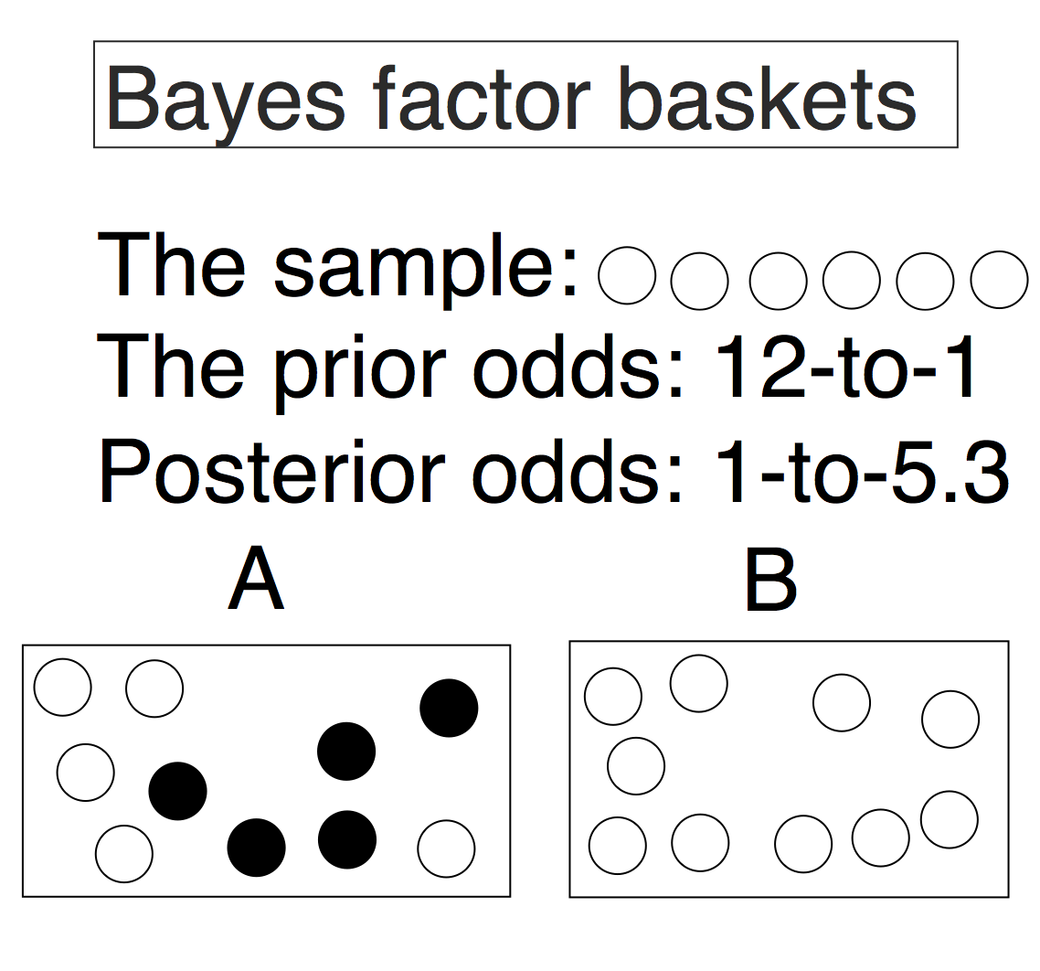
Say you had a different rule for picking the baskets. Let’s say that this time you draw a card and bring me basket B if you draw a King (of any suit) and you bring me basket A if you draw any other card. Now the prior odds are 48-to-4, or 12-to-1, in favor of basket A.
The data from our sample are the same, {W, W, W, W, W, W}, and so is the Bayes factor, 2^6= 64. The conclusion is qualitatively the same, with posterior odds of 1-to-5.3 that favor basket B. This means that, again when considering these as the only two possible baskets, the probability of basket A has been shrunk from 92% to 16% and the probability of basket B has grown from 8% to 84%. The Bayes factor is the same, but we are less confident in our conclusion. The prior odds heavily favored basket A, so it takes more evidence to overcome this handicap and reach as strong a conclusion as before.
What happens when we change the rule once again: Bring me basket B if you draw a King of Hearts and basket A if you draw any other card. Now the prior odds are 51-to-1 in favor of basket A. The data are the same again, and the Bayes factor is still 64. Now the posterior odds are 1-to-1.3 in favor of basket B. This means that the probability of basket A has been shrunk from 98% to 43% and the probability of basket B has grown from 2% to 57%. The evidence, and the Bayes factor, is exactly the same — but the conclusion is totally ambiguous.
Evidence vs. Conclusions
In each case I’ve considered, the evidence has been exactly the same: 6 draws, all white. As a corollary to the discussion above, if you try to come to conclusions based only on the Bayes factor then you are implicitly assuming prior odds of 1-to-1. I think this is unreasonable in most circumstances. When someone looks at a medium-to-large Bayes factor in a study claiming “sadness impairs color perception” (or some other ‘cute’ metaphor study published in Psych Science) and thinks, “I don’t buy this,” they are injecting their prior odds into the equation. Their implicit conclusion is: “My posterior odds for this study are not favorable.” This is the conclusion. The Bayes factor is not the conclusion.
Many studies follow-up on earlier work, so we might give favorable prior odds; thus, when we see a Bayes factor of 5 or 10 we “buy what the study is selling,” so to speak. Or the study might be testing something totally new, so we might give unfavorable prior odds; thus, when we see a Bayes factor of 5 or 10 we remain skeptical. This is just another way of saying that we may reasonably require more evidence for extraordinary claims.
When to stop collecting data
It also follows from the above discussion that sometimes enough is enough. What I mean is that sometimes the conclusion for any reasonable prior odds assignment is strong enough that collecting more data is not worth the time, money, or energy. In the Bayesian framework the stopping rules don’t affect the Bayes factor, and subsequently they don’t affect the posterior odds. Take the second example above, where you gave me basket B if you drew any King. I had prior odds of 12-to-1 in favor of basket A, drew 6 white balls in a row, and ended up with 1-to-5.3 posterior odds in favor of basket B. This translated to a posterior probability of 84% for basket B. If I draw 2 more balls and they are both white, my Bayes factor increases to 2^8=256 (and this should not be corrected for multiple comparisons or so-called “topping up”). My posterior odds increase to roughly 1-to-21 in favor of basket B, and the probability for basket B shoots up from 84% to 99%. I would say that’s enough data for me to make a firm conclusion. But someone else might have other relevant information about the problem I’m studying, and they can come to a different conclusion.
Conclusions are personal
There’s no reason another observer has to come to the same conclusion as me. She might have talked to you and you told her that you actually drew three cards (with replacement and reshuffle) and that you would only have brought me basket B if you drew three kings in a row. She has different information than I do, so naturally she has different prior odds (1728-to-1 in favor of basket A). She would come to a different conclusion than I would, namely that I was actually probably sampling from basket A — her posterior odds are roughly 7-to-1 in favor of basket A. We use the same evidence, a Bayes factor of 2^8=256, but come to different conclusions.
Conclusions are personal. I can’t tell you what to conclude because I don’t know all the information you have access to. But I can tell you what the evidence is, and you can use that to come to your own conclusion. In this post I used a mechanism to generate prior odds that are intuitive and obvious, but we come to our scientific judgments through all sorts of ways that aren’t always easily expressed or quantified. The idea is the same however you come to your prior odds: If you’re skeptical of a study that has a large Bayes factor, then you assigned it strongly unfavorable prior odds.
This is why I, and other Bayesians, advocate for reporting the Bayes factor in experiments. It is not because it tells someone what to conclude from the study, but that it lets them take the information contained in your data to come to their own conclusion. When you report your own Bayes factors for your experiments, in your discussion you might consider how people with different prior odds will react to your evidence. If your Bayes factor is not strong enough to overcome a skeptic’s prior odds, then you may consider collecting more data until it is. If you’re out of resources and the Bayes factor is not strong enough to overcome the prior odds of a moderate skeptic, then there is nothing wrong with acknowledging that other people may reasonably come to different conclusions about your study. Isn’t that how science works?
Bottom line
If you want to come to a conclusion you need the posterior. If you want to make predictions about future sampling you need the posterior. If you want to make decisions you need the posterior (and a utility function; a topic for future blog). If you try to do all this with only the Bayes factor then you are implicitly assuming equal prior odds — which I maintain are almost never appropriate. (Insofar as you do ignore the prior and posterior, then do not be surprised when your Bayes factor simulations find strange results.) In the Bayesian framework each piece has its place. Bayes factors are an important piece of the puzzle, but they are not the only piece. They are simply the most basic piece from my perspective (after the sum and product rules) because they represent the evidence you accumulated in your sample. When you need to do something other than summarize evidence you have to expand your statistical arsenal.
For more introductory material on Bayesian inference, see the Understanding Bayes hub here.
Technical caveat
It’s important to remember that everything is relative and conditional in the Bayesian framework. The posterior probabilities I mention in this post are simply the probabilities of the baskets under the assumption that those are the only relevant hypotheses. They are not absolute probabilities. In other words, instead of writing the posterior probability as P(H|D), it should really be written P(H|D,M), where M is the conditional that the only hypotheses considered are in the following model index: M= {A, B, … K). This is why I personally prefer to use odds notation, since it makes the relativity explicit.
[Edit: There is a now-published Bayesian reanalysis of the RPP. See here.]
The Reproducibility Project was finally published this week in Science, and an outpouring ofmedia articles followed. Headlines included “More Than 50% Psychology Studies Are Questionable: Study”, “Scientists Replicated 100 Psychology Studies, and Fewer Than Half Got the Same Results”, and “More than half of psychology papers are not reproducible”.
Are these categorical conclusions warranted? If you look at the paper, it makes very clear that the results do not definitively establish effects as true or false:
After this intensive effort to reproduce a sample of published psychological findings, how many of the effects have we established are true? Zero. And how many of the effects have we established are false? Zero. Is this a limitation of the project design? No. It is the reality of doing science, even if it is not appreciated in daily practice. (p. 7)
Very well said. The point of this project was not to determine what proportion of effects are “true”. The point of this project was to see what results are replicable in an independent sample.The question arises of what exactly this means. Is an original study replicable if the replication simply matches it in statistical significance and direction? The authors entertain this possibility:
A straightforward method for evaluating replication is to test whether the replication shows a statistically significant effect (P < 0.05) with the same direction as the original study. This dichotomous vote-counting method is intuitively appealing and consistent with common heuristics used to decide whether original studies “worked.” (p. 4)
How did the replications fare? Not particularly well.
Ninety-seven of 100 (97%) effects from original studies were positive results … On the basis of only the average replication power of the 97 original, significant effects [M = 0.92, median (Mdn) = 0.95], we would expect approximately 89 positive results in the replications if all original effects were true and accurately estimated; however, there were just 35 [36.1%; 95% CI = (26.6%, 46.2%)], a significant reduction … (p. 4)
So the replications, being judged on this metric, did (frankly) horribly when compared to the original studies. Only 35 of the studies achieved significance, as opposed to the 89 expected and the 97 total. This gives a success rate of either 36% (35/97) out of all studies, or 39% (35/89) relative to the number of studies expected to achieve significance based on power calculations. Either way, pretty low. These were the numbers that most of the media latched on to.
Does this metric make sense? Arguably not, since the “difference between significant and not significant is not necessarily significant” (Gelman & Stern, 2006). Comparing significance levels across experiments is not valid inference. A non-significant replication result can be entirely consistent with the original effect, and yet count as a failure because it did not achieve significance. There must be a better metric.
The authors recognize this, so they also used a metric that utilized confidence intervals over simple significance tests. Namely, does the confidence interval from the replication study include the originally reported effect? They write,
This method addresses the weakness of the first test that a replication in the same direction and a P value of 0.06 may not be significantly different from the original result. However, the method will also indicate that a replication “fails” when the direction of the effect is the same but the replication effect size is significantly smaller than the original effect size … Also, the replication “succeeds” when the result is near zero but not estimated with sufficiently high precision to be distinguished from the original effect size. (p. 4)
So with this metric a replication is considered successful if the replication result’s confidence interval contains the original effect, and fails otherwise. The replication effect can be near zero, but if the CI is wide enough it counts as a non-failure (i.e., a “success”). A replication can also be quite near the original effect but have high precision, thus excluding the original effect and “failing”.
This metric is very indirect, and their use of scare-quotes around “succeeds” is telling. Roughly 47% of confidence intervals in the replications “succeeded” in capturing the original result. The problem with this metric is obvious: Replications with effects near zero but wide CIs get the same credit as replications that were bang on the original effect (or even larger) with narrow CIs. Results that don’t flat out contradict the original effects count as much as strong confirmations? Why should both of these types of results be considered equally successful?
Based on these two metrics, the headlines are accurate: Over half of the replications “failed”. But these two reproducibility metrics are either invalid (comparing significance levels across experiments) or very vague (confidence interval agreement). They also only offer binary answers: A replication either “succeeds” or “fails”, and this binary thinking leads to absurd conclusions in some cases like those mentioned above. Is replicability really so black and white? I will explain below how I think we should measure replicability in a Bayesian way, with a continuous measure that can find reasonable answers with replication effects near zero with wide CIs, effects near the original with tight CIs, effects near zero with tight CIs, replication effects that go in the opposite direction, and anything in between.
A Bayesian metric of reproducibility
I wanted to look at the results of the reproducibility project through a Bayesian lens. This post should really be titled, “A Bayesian …” or “One Possible Bayesian …” since there is no single Bayesian answer to any question (but those titles aren’t as catchy). It depends on how you specify the problem and what question you ask. When I look at the question of replicability, I want to know if is there evidence for replication success or for replication failure, and how strong that evidence is. That is, should I interpret the replication results as more consistent with the original reported result or more consistent with a null result, and by how much?
Verhagen and Wagenmakers (2014), and Wagenmakers, Verhagen, and Ly (2015) recently outlined how this could be done for many types of problems. The approach naturally leads to computing a Bayes factor. With Bayes factors, one must explicitly define the hypotheses (models) being compared. In this case one model corresponds to a probability distribution centered around the original finding (i.e. the posterior), and the second model corresponds to the null model (effect = 0). The Bayes factor tells you which model the replication result is more consistent with, and larger Bayes factors indicate a better relative fit. So it’s less about obtaining evidence for the effect in general and more about gauging the relative predictive success of the original effects. (footnote 1)
If the original results do a good job of predicting replication results, the original effect model will achieve a relatively large Bayes factor. If the replication results are much smaller or in the wrong direction, the null model will achieve a large Bayes factor. If the result is ambiguous, there will be a Bayes factor near 1. Again, the question is which model better predicts the replication result? You don’t want a null model to predict replication results better than your original reported effect.
A key advantage of the Bayes factor approach is that it allows natural grades of evidence for replication success. A replication result can strongly agree with the original effect model, it can strongly agree with a null model, or it can lie somewhere in between. To me, the biggest advantage of the Bayes factor is it disentangles the two types of results that traditional significance tests struggle with: a result that actually favors the null model vs a result that is simply insensitive. Since the Bayes factor is inherently a comparative metric, it is possible to obtain evidence for the null model over the tested alternative. This addresses my problem I had with the above metrics: Replication results bang on the original effects get big boosts in the Bayes factor, replication results strongly inconsistent with the original effects get big penalties in the Bayes factor, and ambiguous replication results end up with a vague Bayes factor.
Bayes factor methods are often criticized for being subjective, sensitive to the prior, and for being somewhat arbitrary. Specifying the models is typically hard, and sometimes more arbitrary models are chosen for convenience for a given study. Models can also be specified by theoretical considerations that often appear subjective (because they are). For a replication study, the models are hardly arbitrary at all. The null model corresponds to that of a skeptic of the original results, and the alternative model corresponds to a strong theoretical proponent. The models are theoretically motivated and answer exactly what I want to know: Does the replication result fit more with the original effect model or a null model? Or as Verhagen and Wagenmakers (2014) put it, “Is the effect similar to what was found before, or is it absent?” (p.1458 here).
Replication Bayes factors
In the following, I take the effects reported in figure 3 of the reproducibility project (the pretty red and green scatterplot) and calculate replication Bayes factors for each one. Since they have been converted to correlation measures, replication Bayes factors can easily be calculated using the code provided by Wagenmakers, Verhagen, and Ly (2015). The authors of the reproducibility project kindly provide the script for making their figure 3, so all I did was take the part of the script that compiled the converted 95 correlation effect sizes for original and replication studies. (footnote 2) The replication Bayes factor script takes the correlation coefficients from the original studies as input, calculates the corresponding original effect’s posterior distribution, and then compares the fit of this distribution and the null model to the result of the replication. Bayes factors larger than 1 indicate the original effect model is a better fit, Bayes factors smaller than 1 indicate the null model is a better fit. Large (or really small) Bayes factors indicate strong evidence, and Bayes factors near 1 indicate a largely insensitive result.
The replication Bayes factors are summarized in the figure below (click to enlarge). The y-axis is the count of Bayes factors per bin, and the different bins correspond to various strengths of replication success or failure. Results that fall in the bins left of center constitute support the null over the original result, and vice versa. The outer-most bins on the left or right contain the strongest replication failures and successes, respectively. The bins labelled “Moderate” contain the more muted replication successes or failures. The two central-most bins labelled “Insensitive” contain results that are essentially uninformative.
So how did we do?
You’ll notice from this crude binning system that there is quite a spread from super strong replication failure to super strong replication success. I’ve committed the sin of binning a continuous outcome, but I think it serves as a nice summary. It’s important to remember that Bayes factors of 2.5 vs 3.5, while in different bins, aren’t categorically different. Bayes factors of 9 vs 11, while in different bins, aren’t categorically different. Bayes factors of 15 and 90, while in the same bin, are quite different. There is no black and white here. These are the categories Bayesians often use to describe grades of Bayes factors, so I use them since they are familiar to many readers. If you have a better idea for displaying this please leave a comment. 🙂 Check out the “Results” section at the end of this post to see a table which shows the study number, the N in original and replications, the r values of each study, the replication Bayes factor and category I gave it, and the replication p-value for comparison with the Bayes factor. This table shows the really wide spread of the results. There is also code in the “Code” section to reproduce the analyses.
Strong replication failures and strong successes
Roughly 20% (17 out of 95) of replications resulted in relatively strong replication failures (2 left-most bins), with resultant Bayes factors at least 10:1 in favor of the null. The highest Bayes factor in this category was over 300,000 (study 110, “Perceptual mechanisms that characterize gender differences in decoding women’s sexual intent”). If you were skeptical of these original effects, you’d feel validated in your skepticism after the replications. If you were a proponent of the original effects’ replicability you’ll perhaps want to think twice before writing that next grant based around these studies.
Roughly 25% (23 out of 95) of replications resulted in relatively strong replication successes (2 right-most bins), with resultant Bayes factors at least 10:1 in favor of the original effect. The highest Bayes factor in this category was 1.3×10^32 (or log(bf)=74; study 113, “Prescribed optimism: Is it right to be wrong about the future?”) If you were a skeptic of the original effects you should update your opinion to reflect the fact that these findings convincingly replicated. If you were a proponent of these effects you feel validation in that they appear to be robust.
These two types of results are the most clear-cut: either the null is strongly favored or the original reported effect is strongly favored. Anyone who was indifferent to these effects has their opinion swayed to one side, and proponents/skeptics are left feeling either validated or starting to re-evaluate their position. There was only 1 very strong (BF>100) failure to replicate but there were quite a few very strong replication successes (16!). There were approximately twice as many strong (10<BF<100) failures to replicate (16) than strong replication successes (7).
Moderate replication failures and moderate successes
The middle-inner bins are labelled “Moderate”, and contain replication results that aren’t entirely convincing but are still relatively informative (3<BF<10). The Bayes factors in the upper end of this range are somewhat more convincing than the Bayes factors in the lower end of this range.
Roughly 20% (19 out of 95) of replications resulted in moderate failures to replicate (third bin from the left), with resultant Bayes factors between 10:1 and 3:1 in favor of the null. If you were a proponent of these effects you’d feel a little more hesitant, but you likely wouldn’t reconsider your research program over these results. If you were a skeptic of the original effects you’d feel justified in continued skepticism.
Roughly 10% (9 out of 95) of replications resulted in moderate replication successes (third bin from the right), with resultant Bayes factors between 10:1 and 3:1 in favor of the original effect. If you were a big skeptic of the original effects, these replication results likely wouldn’t completely change your mind (perhaps you’d be a tad more open minded). If you were a proponent, you’d feel a bit more confident.
Many uninformative “failed” replications
The two central bins contain replication results that are insensitive. In general, Bayes factors smaller than 3:1 should be interpreted only as very weak evidence. That is, these results are so weak that they wouldn’t even be convincing to an ideal impartial observer (neither proponent nor skeptic). These two bins contain 27 replication results. Approximately 30% of the replication results from the reproducibility project aren’t worth much inferentially!
A few examples:
Study 2, “Now you see it, now you don’t: repetition blindness for nonwords” BF = 2:1 in favor of null
Study 12, “When does between-sequence phonological similarity promote irrelevant sound disruption?” BF = 1.1:1 in favor of null
Study 80, “The effects of an implemental mind-set on attitude strength.” BF = 1.2:1 in favor of original effect
Study 143, “Creating social connection through inferential reproduction: Loneliness and perceived agency in gadgets, gods, and greyhounds” BF = 2:1 in favor of null
I just picked these out randomly. The types of replication studies in this inconclusive set range from attentional blink (study 2), to brain mapping studies (study 55), to space perception (study 167), to cross national comparisons of personality (study 154).
Should these replications count as “failures” to the same extent as the ones in the left 2 bins? Should studies with a Bayes factor of 2:1 in favor of the original effect count as “failures” as much as studies with 50:1 against? I would argue they should not, they should be called what they are: entirely inconclusive.
Interestingly, study 143 mentioned above was recently called out in this NYT article as a high-profile study that “didn’t hold up”. Actually, we don’t know if it held up! Identifying replications that were inconclusive using this continuous range helps avoid over-interpreting ambiguous results as “failures”.
Wrap up
To summarize the graphic and the results discussed above, this method identifies roughly as many replications with moderate success or better (BF>3) as the counting significance method (32 vs 35). (footnote 3) These successes can be graded based on their replication Bayes factor as moderate to very strong. The key insight from using this method is that many replications that “fail” based on the significance count are actually just inconclusive. It’s one thing to give equal credit to two replication successes that are quite different in strength, but it’s another to call all replications failures equally bad when they show a highly variable range. Calling a replication a failure when it is actually inconclusive has consequences for the original researcher and the perception of the field.
As opposed to the confidence interval metric, a replication effect centered near zero with a wide CI will not count as a replication success with this method; it would likely be either inconclusive or weak evidence in favor of the null. Some replications are indeed moderate to strong failures to replicate (36 or so), but nearly 30% of all replications in the reproducibility project (27 out of 95) were not very informative in choosing between the original effect model and the null model.
So to answer my question as I first posed it, are the categorical conclusions of wide-scale failures to replicate by the media stories warranted? As always, it depends.
If you count “success” as any Bayes factor that has any evidence in favor of the original effect (BF>1), then there is a 44% success rate (42 out of 95).
If you count “success” as any Bayes factor with at least moderate evidence in favor of the original effect (BF>3), then there is a 34% success rate (32 out of 95).
If you count “failure” as any Bayes factor that has at least moderate evidence in favor of the null (BF<1/3), then there is a 38% failure rate (36 out of 95).
If you only consider the effects sensitive enough to discriminate the null model and the original effect model (BF>3 or BF<1/3) in your total, then there is a roughly 47% success rate (32 out of 68). This number jives (uncannily) well with the prediction John Ioannidis made 10 years ago (47%).
However you judge it, the results aren’t exactly great.
But if we move away from dichotomous judgements of replication success/failure, we see a slightly less grim picture. Many studies strongly replicated, many studies strongly failed, but many studies were in between. There is a wide range! Judgements of replicability needn’t be black and white. And with more data the inconclusive results could have gone either way. I would argue that any study with 1/3<BF<3 shouldn’t count as a failure or a success, since the evidence simply is not convincing; I think we should hold off judging these inconclusive effects until there is stronger evidence. Saying “we didn’t learn much about this or that effect” is a totally reasonable thing to do. Boo dichotomization!
Try out this method!
All in all, I think the Bayesian approach to evaluating replication success is advantageous in 3 big ways: It avoids dichotomizing replication outcomes, it gives an indication of the range of the strength of replication successes or failures, and it identifies which studies we need to give more attention to (insensitive BFs). The Bayes factor approach used here can straighten out when a replication shows strong evidence in favor of the null model, strong evidence in favor of the original effect model, or evidence that isn’t convincingly in favor of either position. Inconclusive replications should be targeted for future replication, and perhaps we should look into why these studies that purport to have high power (>90%) end up with insensitive results (large variance, design flaw, overly optimistic power calcs, etc). It turns out that having high power in planning a study is no guarantee that one actually obtains convincingly sensitive data (Dienes, 2014; Wagenmakers et al., 2014).
I should note, the reproducibility project did try to move away from the dichotomous thinking about replicability by correlating the converted effect sizes (r) between original and replication studies. This was a clever idea, and it led to a very pretty graph (figure 3) and some interesting conclusions. That idea is similar in spirit to what I’ve laid out above, but its conclusions can only be drawn from batches of replication results. Replication Bayes factors allow one to compare the original and replication results on an effect by effect basis. This Bayesian method can grade a replication on its relative success or failure even if your reproducibility project only has 1 effect in it.
I should also note, this analysis is inherently context dependent. A different group of studies could very well show a different distribution of replication Bayes factors, where each individual study has a different prior distribution (based on the original effect). I don’t know how much these results would generalize to other journals or other fields, but I would be interested to see these replication Bayes factors employed if systematic replication efforts ever do catch on in other fields.
Acknowledgements and thanks
The authors of the reproducibility project have done us all a great service and I am grateful that they have shared all of their code, data, and scripts. This re-analysis wouldn’t have been possible without their commitment to open science. I am also grateful to EJ Wagenmakers, Josine Verhagen, and Alexander Ly for sharing the code to calculate the replication Bayes factors on the OSF. Many thanks to Chris Engelhardt and Daniel Lakens for some fruitful discussions when I was planning this post. Of course, the usual disclaimer applies and all errors you find should be attributed only to me.
Notes
footnote 1: Of course, a model that takes publication bias into account could fit better by tempering the original estimate, and thus show relative evidence for the bias-corrected effect vs either of the other models; but that’d be answering a different question than the one I want to ask.
footnote 2: I left out 2 results that I couldn’t get to work with the calculations. Studies 46 and 139, both appear to be fairly strong successes, but I’ve left them out of the reported numbers because I couldn’t calculate a BF.
footnote 3: The cutoff of BF>3 isn’t a hard and fast rule at all. Recall that this is a continuous measure. Bayes factors are typically a little more conservative than significance tests in supporting the alternative hypothesis. If the threshold for success is dropped to BF>2 the number of successes is 35 — an even match with the original estimate.
Results
This table is organized from smallest replication Bayes factor to largest (i.e., strongest evidence in favor of null to strongest evidence in favor of original effect). The Ns were taken from the final columns in the master data sheet,”T_N_O_for_tables” and “T_N_R_for_tables”. Some Ns are not integers because they presumably underwent df correction. There is also the replication p-value for comparison; notice that BFs>3 generally correspond to ps less than .05 — BUT there are some cases where they do not agree. If you’d like to see more about the studies you can check out the master data file in the reproducibility project OSF page (linked below).
This file contains hidden or bidirectional Unicode text that may be interpreted or compiled differently than what appears below. To review, open the file in an editor that reveals hidden Unicode characters.
Learn more about bidirectional Unicode characters
If you want to check/modify/correct my code, here it is. If you find a glaring error please leave a comment below or tweet at me 🙂
This file contains hidden or bidirectional Unicode text that may be interpreted or compiled differently than what appears below. To review, open the file in an editor that reveals hidden Unicode characters.
Learn more about bidirectional Unicode characters
Dienes, Z. (2014). Using Bayes to get the most out of non-significant results. Frontiers in psychology, 5.
Gelman, A., & Stern, H. (2006). The difference between “significant” and “not significant” is not itself statistically significant. The American Statistician, 60(4), 328-331.
Open Science Collaboration (2015). Estimating the reproducibility of psychological science. Science 28 August 2015: 349 (6251), aac4716 [DOI:10.1126/science.aac4716]
Verhagen, J., & Wagenmakers, E. J. (2014). Bayesian tests to quantify the result of a replication attempt. Journal of Experimental Psychology: General,143(4), 1457.
Wagenmakers, E. J., Verhagen, A. J., & Ly, A. (in press). How to quantify the evidence for the absence of a correlation. Behavior Research Methods.
Wagenmakers, E. J., Verhagen, J., Ly, A., Bakker, M., Lee, M. D., Matzke, D., … & Morey, R. D. (2014). A power fallacy. Behavior research methods, 1-5.
In the first post of the Understanding Bayes series I said:
The likelihood is the workhorse of Bayesian inference. In order to understand Bayesian parameter estimation you need to understand the likelihood. In order to understand Bayesian model comparison (Bayes factors) you need to understand the likelihood and likelihood ratios.
I’ve shown in another post how the likelihood works as the updating factor for turning priors into posteriors for parameter estimation. In this post I’ll explain how using Bayes factors for model comparison can be conceptualized as a simple extension of likelihood ratios.
There’s that coin again
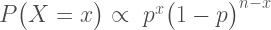
Imagine we’re in a similar situation as before: I’ve flipped a coin 100 times and it came up 60 heads and 40 tails. The likelihood function for binomial data in general is:
and for this particular result:
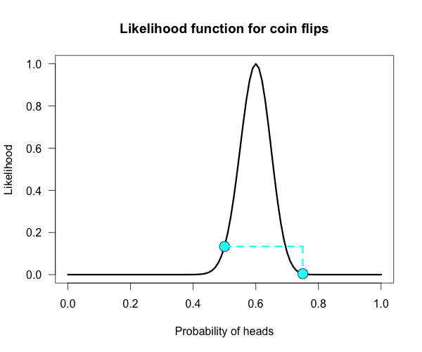
The corresponding likelihood curve is shown below, which displays the relative likelihood for all possible simple (point) hypotheses given this data. Any likelihood ratio can be calculated by simply taking the ratio of the different hypotheses’s heights on the curve.
In that previous post I compared the fair coin hypothesis — H0: P(H)=.5 — vs one particular trick coin hypothesis — H1: P(H)=.75. For 60 heads out of 100 tosses, the likelihood ratio for these hypotheses is L(.5)/L(.75) = 29.9. This means the data are 29.9 times as probable under the fair coin hypothesis than this particular trick coin hypothesis. But often we don’t have theories precise enough to make point predictions about parameters, at least not in psychology. So it’s often helpful if we can assign a range of plausible values for parameters as dictated by our theories.
Enter the Bayes factor
Calculating a Bayes factor is a simple extension of this process. A Bayes factor is a weighted average likelihood ratio, where the weights are based on the prior distribution specified for the hypotheses. For this example I’ll keep the simple fair coin hypothesis as the null hypothesis — H0: P(H)=.5 — but now the alternative hypothesis will become a composite hypothesis — H1: P(θ). (footnote 1) The likelihood ratio is evaluated at each point of P(θ) and weighted by the relative plausibility we assign that value. Then once we’ve assigned weights to each ratio we just take the average to get the Bayes factor. Figuring out how the weights should be assigned (the prior) is the tricky part.
Imagine my composite hypothesis, P(θ), is a combination of 21 different point hypotheses, all evenly spaced out between 0 and 1 and all of these points are weighted equally (not a very realistic hypothesis!). So we end up with P(θ) = {0, .05, .10, .15, . . ., .9, .95, 1}. The likelihood ratio can be evaluated at every possible point hypothesis relative to H0, and we need to decide how to assign weights. This is easy for this P(θ); we assign zero weight for every likelihood ratio that is not associated with one of the point hypotheses contained in P(θ), and we assign weights of 1 to all likelihood ratios associated with the 21 points in P(θ).
This gif has the 21 point hypotheses of P(θ) represented as blue vertical lines (indicating where we put our weights of 1), and the turquoise tracking lines represent the likelihood ratio being calculated at every possible point relative to H0: P(H)=.5. (Remember, the likelihood ratio is the ratio of the heights on the curve.) This means we only care about the ratios given by the tracking lines when the dot attached to the moving arm aligns with the vertical P(θ) lines. [edit: this paragraph added as clarification]
The 21 likelihood ratios associated with P(θ) are:
Since they are all weighted equally we simply average, and obtain BF = 18.3/21 = .87. In other words, the data (60 heads out of 100) are 1/.87 = 1.15 times more probable under the null hypothesis — H0: P(H)=.5 — than this particular composite hypothesis — H1: P(θ). Entirely uninformative! Despite tossing the coin 100 times we have extremely weak evidence that is hardly worth even acknowledging. This happened because much of P(θ) falls in areas of extremely low likelihood relative to H0, as evidenced by those 13 zeros above. P(θ) is flexible, since it covers the entire possible range of θ, but this flexibility comes at a price. You have to pay for all of those zeros with a lower weighted average and a smaller Bayes factor.
Now imagine I had seen a trick coin like this before, and I know it had a slight bias towards landing heads. I can use this information to make more pointed predictions. Let’s say I define P(θ) as 21 equally weighted point hypotheses again, but this time they are all equally spaced between .5 and .75, which happens to be the highest density region of the likelihood curve (how fortuitous!). Now P(θ) = {.50, .5125, .525, . . ., .7375, .75}.
The 21 likelihood ratios associated with the new P(θ) are:
They are all still weighted equally, so the simple average is BF = 72/21 = 3.4. Three times more informative than before, and in favor of P(θ) this time! Andno zeros. We were able to add theoretically relevant information to H1 to make more accurate predictions, and we get rewarded with a Bayes boost. (But this result is only 3-to-1 evidence, which is still fairly weak.)
This new P(θ) is risky though, because if the data show a bias towards tails or a more extreme bias towards heads then it faces a very heavy penalty (many more zeros). High risk = high reward with the Bayes factor. Make pointed predictions that match the data and get a bump to your BF, but if you’re wrong then pay a steep price. For example, if the data were 60 tails instead of 60 heads the BF would be 10-to-1 against P(θ) rather than 3-to-1 for P(θ)!
Now, typically people don’t actually specify hypotheses like these. Typically they use continuous distributions, but the idea is the same. Take the likelihood ratio at each point relative to H0, weigh according to plausibilities given in P(θ), and then average.
A more realistic (?) example
Imagine you’re walking down the sidewalk and you see a shiny piece of foreign currency by your feet. You pick it up and want to know if it’s a fair coin or an unfair coin. As a Bayesian you have to be precise about what you mean by fair and unfair. Fair is typically pretty straightforward — H0: P(H)=.5 as before — but unfair could mean anything. Since this is a completely foreign coin to you, you may want to be fairly open-minded about it. After careful deliberation, you assign P(θ) a beta distribution, with shape parameters 10 and 10. That is, H1: P(θ) ~ Beta(10, 10). This means that if the coin isn’t fair, it’s probably close to fair but it could reasonably be moderately biased, and you have no reason to think it is particularly biased to one side or the other.
Now you build a perfect coin-tosser machine and set it to toss 100 times (but not any more than that because you haven’t got all day). You carefully record the results and the coin comes up 33 heads out of 100 tosses. Under which hypothesis are these data more probable, H0 or H1? In other words, which hypothesis did the better job predicting these data?
This may be a continuous prior but the concept is exactly the same as before: weigh the various likelihood ratios based on the prior plausibility assignment and then average. The continuous distribution on P(θ) can be thought of as a set of many many point hypotheses spaced very very close together. So if the range of θ we are interested in is limited to 0 to 1, as with binomials and coin flips, then a distribution containing 101 point hypotheses spaced .01 apart, can effectively be treated as if it were continuous. The numbers will be a little off but all in all it’s usually pretty close. So imagine that instead of 21 hypotheses you have 101, and their relative plausibilities follow the shape of a Beta(10, 10). (footnote 2)
Since this is not a uniform distribution, we need to assign varying weights to each likelihood ratio. Each likelihood ratio associated with a point in P(θ) is simply multiplied by the respective density assigned to it under P(θ). For example, the density of P(θ) at .4 is 2.44. So we multiply the likelihood ratio at that point, L(.4)/L(.5) = 128, by 2.44, and add it to the accumulating total likelihood ratio. Do this for every point and then divide by the total number of points, in this case 101, to obtain the approximate Bayes factor. The total weighted likelihood ratio is 5564.9, divide it by 101 to get 55.1, and there’s the Bayes factor. In other words, the data are roughly 55 times more probable under this composite H1 than under H0. The alternative hypothesis H1 did a much better job predicting these data than did the null hypothesis H0.
The actual Bayes factor is obtained by integrating the likelihood with respect to H1’s density distribution and then dividing by the (marginal) likelihood of H0. Essentially what it does is cut P(θ) into slices infinitely thin before it calculates the likelihood ratios, re-weighs, and averages. That Bayes factor comes out to 55.7, which is basically the same thing we got through this ghetto visualization demonstration!
Take home
The take-home message is hopefully pretty clear at this point: When you are comparing a point null hypothesis with a composite hypothesis, the Bayes factor can be thought of as a weighted average of every point hypothesis’s likelihood ratio against H0, and the weights are determined by the prior density distribution of H1. Since the Bayes factor is a weighted average based on the prior distribution, it’s really important to think hard about the prior distribution you choose for H1. In a previous post, I showed how different priors can converge to the same posterior with enough data. The priors are often said to “wash out” in estimation problems like that. This is not necessarily the case for Bayes factors. The priors you choose matter, so think hard!
Notes
Footnote 1: A lot of ink has been spilled arguing about how one should define P(θ). I talked about it a little a previous post.
Footnote 2: I’ve rescaled the likelihood curve to match the scale of the prior density under H1. This doesn’t affect the values of the Bayes factor or likelihood ratios because the scaling constant cancels itself out.
R code
This file contains hidden or bidirectional Unicode text that may be interpreted or compiled differently than what appears below. To review, open the file in an editor that reveals hidden Unicode characters.
Learn more about bidirectional Unicode characters