[Some material from this post has been incorporated into a paper to be published in AMPPS]
In a previous post I outlined the basic idea behind likelihoods and likelihood ratios. Likelihoods are relatively straightforward to understand because they are based on tangible data. Collect your data, and then the likelihood curve shows the relative support that your data lend to various simple hypotheses. Likelihoods are a key component of Bayesian inference because they are the bridge that gets us from prior to posterior.
In this post I explain how to use the likelihood to update a prior into a posterior. The simplest way to illustrate likelihoods as an updating factor is to use conjugate distribution families (Raiffa & Schlaifer, 1961). A prior and likelihood are said to be conjugate when the resulting posterior distribution is the same type of distribution as the prior. This means that if you have binomial data you can use a beta prior to obtain a beta posterior. If you had normal data you could use a normal prior and obtain a normal posterior. Conjugate priors are not required for doing bayesian updating, but they make the calculations a lot easier so they are nice to use if you can.
I’ll use some data from a recent NCAA 3-point shooting contest to illustrate how different priors can converge into highly similar posteriors.
The data
This year’s NCAA shooting contest was a thriller that saw Cassandra Brown of the Portland Pilots win the grand prize. This means that she won the women’s contest and went on to defeat the men’s champion in a shoot-off. This got me thinking, just how good is Cassandra Brown?
What a great chance to use some real data in a toy example. She completed 4 rounds of shooting, with 25 shots in each round, for a total of 100 shots (I did the math). The data are counts, so I’ll be using the binomial distribution as a data model (i.e., the likelihood. See this previous post for details). Her results were the following:
Round 1: 13/25 Round 2: 12/25 Round 3: 14/25 Round 4: 19/25
Total: 58/100
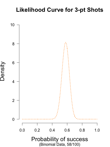
The likelihood curve below encompasses the entirety of statistical evidence that our 3-point data provide (footnote 1). The hypothesis with the most relative support is .58, and the curve is moderately narrow since there are quite a few data points. I didn’t standardize the height of the curve in order to keep it comparable to the other curves I’ll be showing.
The prior
Now the part that people often make a fuss about: choosing the prior. There are a few ways to choose a prior. Since I am using a binomial likelihood, I’ll be using a conjugate beta prior. A beta prior has two shape parameters that determine what it looks like, and is denoted Beta(α, β). I like to think of priors in terms of what kind of information they represent. The shape parameters α and β can be thought of as prior observations that I’ve made (or imagined).
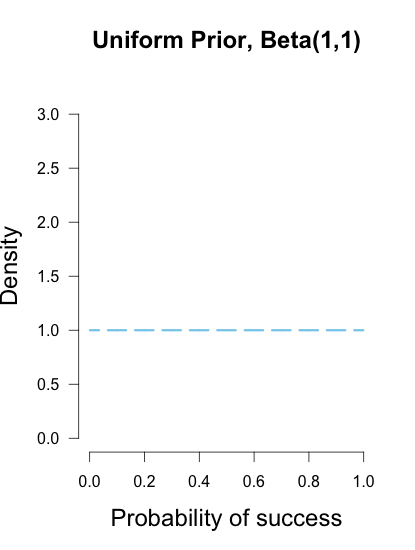
Imagine my trusted friend caught the end of Brown’s warm-up and saw her take two shots, making one and missing the other, and she tells me this information. This would mean I could reasonably use the common Beta(1, 1) prior, which represents a uniform density over [0, 1]. In other words, all possible values for Brown’s shooting percentage are given equal weight before taking data into account, because the only thing I know about her ability is that both outcomes are possible (Lee & Wagenmakers, 2005).
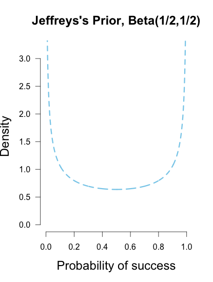
Another common prior is called Jeffreys’s prior, a Beta(1/2, 1/2) which forms a wide bowl shape. This prior would be recommended if you had extremely scarce information about Brown’s ability. Is Brown so good that she makes nearly every shot, or is she so bad that she misses nearly every shot? This prior says that Brown’s shooting rate is probably near the extremes, which may not necessarily reflect a reasonable belief for someone who is a college basketball player, but it has the benefit of having less influence on the posterior estimates than the uniform prior (since it is equal to 1 prior observation instead of 2). Jeffreys’s prior is popular because it has some desirable properties, such as invariance under parameter transformation (Jaynes, 2003). So if instead of asking about Brown’s shooting percentage I instead wanted to know her shooting percentage squared or cubed, Jeffreys’s prior would remain the same shape while many other priors would drastically change shape.
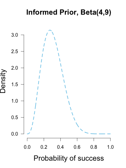
Or perhaps I had another trusted friend who had arrived earlier and seen Brown take her final 13 shots in warm-up, and she saw 4 makes and 9 misses. Then I could use a Beta(4, 9) prior to characterize this prior information, which looks like a hump over .3 with density falling slowly as it moves outward in either direction. This prior has information equivalent to 13 shots, or roughly an extra 1/2 round of shooting.
These three different priors are shown below.
These are but three possible priors one could use. In your analysis you can use any prior you want, but if you want to be taken seriously you’d better give some justification for it. Bayesian inference allows many rules for prior construction.”This is my personal prior” is a technically a valid reason, but if this is your only justification then your colleagues/reviewers/editors will probably not take your results seriously.
Updating the prior via the likelihood
Now for the easiest part. In order to obtain a posterior, simply use Bayes’s rule:

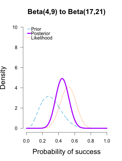
The posterior is proportional to the likelihood multiplied by the prior. What’s nice about working with conjugate distributions is that Bayesian updating really is as simple as basic algebra. We take the formula for the binomial likelihood, which from a previous post is known to be:

and then multiply it by the formula for the beta prior with α and β shape parameters:
to obtain the following formula for the posterior:

With a little bit of algebra knowledge, you’ll know that multiplying together terms with the same base means the exponents can be added together. So the posterior formula can be rewritten as:

and then by adding the exponents together the formula simplifies to:

and it’s that simple! Take the prior, add the successes and failures to the different exponents, and voila. The distributional notation is even simpler. Take the prior, Beta(α, β), and add the successes from the data, x, to α and the failures, n – x, to β, and there’s your posterior, Beta(α+x, β+n-x).
Remember from the previous post that likelihoods don’t care about what order the data arrive in, it always results in the same curve. This property of likelihoods is carried over to posterior updating. The formulas above serve as another illustration of this fact. It doesn’t matter if you add a string of six single data points, 1+1+1+1+1+1+1 or a batch of +6 data points; the posterior formula in either case ends up with 6 additional points in the exponents.
Looking at some posteriors
Back to Brown’s shooting data. She had four rounds of shooting so I’ll treat each round as a batch of new data. Her results for each round were: 13/25, 12/25, 14/25, 19/25. I’ll show how the different priors are updated with each batch of data. A neat thing about bayesian updating is that after batch 1 is added to the initial prior, its posterior is used as the prior for the next batch of data. And as the formulas above indicate, the order or frequency of additions doesn’t make a difference on the final posterior. I’ll verify this at the end of the post.
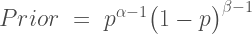
In the following plots, the prior is shown in blue (as above), the likelihood in orange (as above), and the resulting posteriors after Brown’s first 13/25 makes in purple.
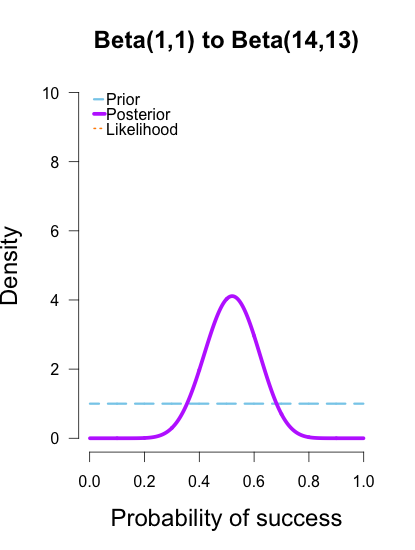
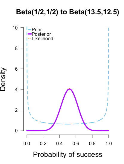
In the first and second plot the likelihood is nearly invisible because the posterior sits right on top of it. When the prior has only 1 or 2 data points worth of information, it has essentially no impact on the posterior shape (footnote 2). The third plot shows how the posterior splits the difference between the likelihood and the informed prior based on the relative quantity of information in each.
The posteriors obtained from the uniform and Jeffreys’s priors suggest the best guess for Brown’s shooting percentage is around 50%, whereas the posterior obtained from the informed prior suggests it is around 40%. No surprise here since the informed prior represents another 1/2 round of shots where Brown performed poorly, which shifts the posterior towards lower values. But all three posteriors are still quite broad, and the breadth of the curves can be thought to represent the uncertainty in my estimates. More data -> tighter curves -> less uncertainty.
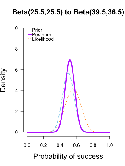
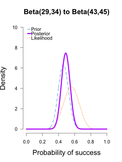
Now I’ll add the second round performance as a new likelihood (12/25 makes), and I’ll take the posteriors from the first round of updating as new priors for the second round of updating. So the purple posteriors from the plots above are now blue priors, the likelihood is orange again, and the new posteriors are purple.
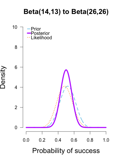
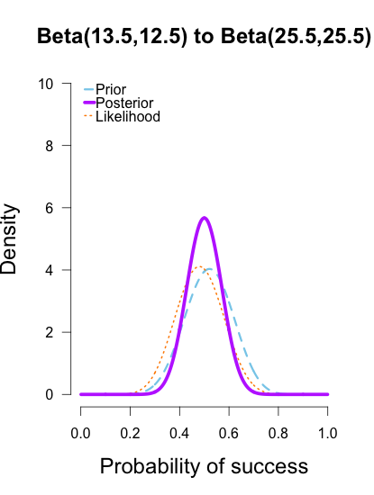
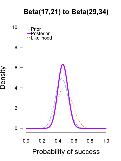
The left two plots look nearly identical, which should be no surprise since their posteriors were essentially equivalent after only 1 round of data updates. The third plot shows a posterior still slightly shifted to the left of the others, but it is much more in line with them than before. All three posteriors are getting narrower as more data is added.
The last two rounds of updating are shown below, again with posteriors from the previous round taken as priors for the next round. At this point they’ve all converged to very similar posteriors that are much narrower, translating to less uncertainty in my estimates.
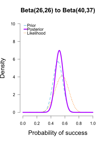
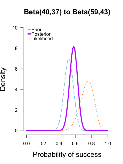
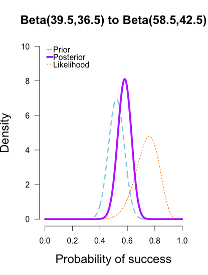
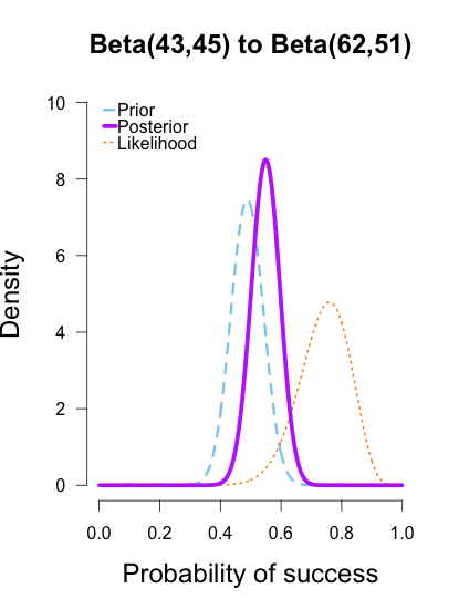
These posterior distributions look pretty similar now! Just as an illustration, I’ll show what happens when I update the initial priors with all of the data at once.
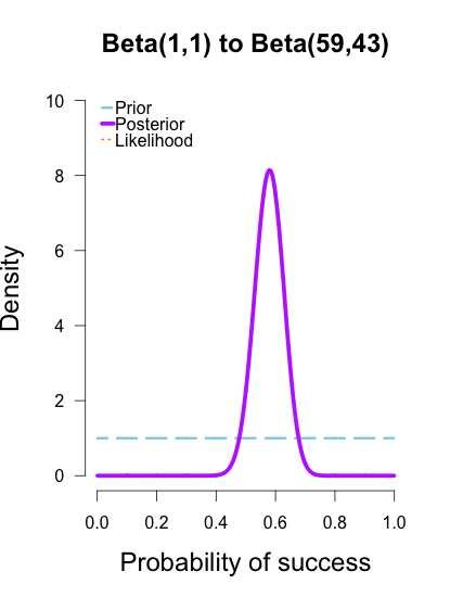
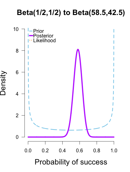
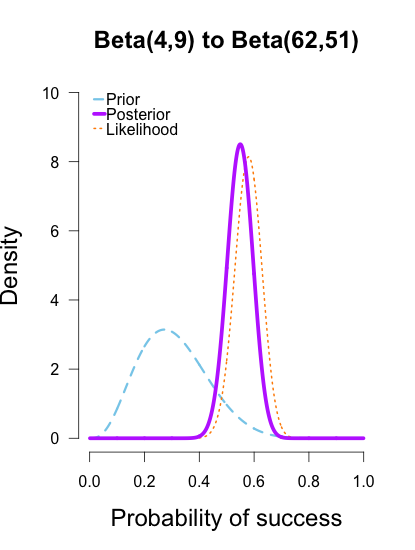
As the formulas predict, the posteriors after one big batch of data are identical to those obtained by repeatedly adding multiple smaller batches of data. It’s also a little easier to see the discrepancies between the final posteriors in this illustration because the likelihood curve acts as a visual anchor. The uniform and Jeffreys’s priors result in posteriors that essentially fall right on top of the likelihood, whereas the informed prior results in a posterior that is very slightly shifted to the left of the likelihood.
My takeaway from these posteriors is that Cassandra Brown has a pretty damn good 3-point shot! In a future post I’ll explain how to use this method of updating to make inferences using Bayes factors. It’s called the Savage-Dickey density method, and I think it’s incredibly intuitive and easy to use.
Notes:
Footnote 1: I’m making a major assumption about the data: Any one shot is exchangeable with any other shot. This might not be defensible since the final ball on each rack is worth a bonus point, so maybe those shots differ systematically from regular shots, but it’s a toy example so I’ll ignore that possibility. There’s also the possibility of her going on a hot streak, a.k.a. having a “hot hand”, but I’m going to ignore that too because I’m the one writing this blog post and I want to keep it simple. There’s also the possibility that she gets worse throughout the competition because she gets tired, but then there’s also the possibility that she gets better as she warms up with multiple rounds. All of these things are reasonable to consider and I am going to ignore them all.
Footnote 2: There is a tendency to call any priors that have very little impact on the posterior “non-informative”, but, as I mentioned in the section on determining priors, uniform priors that seem non-informative in one context can become highly informative with parameter transformation (Zhu & Lu, 2004). Jeffreys’s prior was derived precisely with that in mind, so it carries little information no matter what transformation is applied.
R Code
| shotData<- c(1, 0, 0, 0, 1, 0, 1, 0, 1, 0, 0, 0, 1, 1, 1, 0, 1, 0, 1, 1, 1, 0, 0, 1, 1, 0, 0, | |
| 1, 1, 1, 0, 0, 1, 1, 0, 0, 0, 1, 1, 1, 0, 0, 0, 0, 1, 1, 0, 1, 1, 0, 1, 0, 0, 1, | |
| 0, 1, 0, 1, 1, 1, 0, 1, 0, 1, 0, 0, 1, 1, 0, 1, 0, 0, 1, 1, 1, 1, 1, 1, 1, 1, 1, | |
| 1, 1, 1, 0, 0, 1, 1, 0, 0, 1, 1, 1, 0, 1, 1, 1, 1, 1, 0) | |
| #figure 1 from blog, likelihood curve for 58/100 shots | |
| x = seq(.001, .999, .001) ##Set up for creating the distributions | |
| y2 = dbeta(x, 1 + 58, 1 + 42) # data for likelihood curve, plotted as the posterior from a beta(1,1) | |
| plot(x, y2, xlim=c(0,1), ylim=c(0, 1.25 * max(y2,1.6)), type = "l", ylab= "Density", lty = 3, | |
| xlab= "Probability of success", las=1, main="Likelihood Curve for 3-pt Shots", sub= "(Binomial Data, 58/100)",lwd=2, | |
| cex.lab=1.5, cex.main=1.5, col = "darkorange", axes=FALSE) | |
| axis(1, at = seq(0,1,.2)) #adds custom x axis | |
| axis(2, las=1) # custom y axis | |
| ## Function for plotting priors, likelihoods, and posteriors for binomial data | |
| ## Output consists of a plot and various statistics | |
| ## PS and PF determine the shape of the prior distribution. | |
| ## PS = prior success, PF = prior failure for beta dist. | |
| ## PS = 1, PF = 1 corresponds to uniform(0,1) and is default. If left at default, posterior will be equivalent to likelihood | |
| ## k = number of observed successes in the data, n = total trials. If left at 0 only plots the prior dist. | |
| ## null = Is there a point-null hypothesis? null = NULL leaves it out of plots and calcs | |
| ## CI = Is there a relevant X% credibility interval? .95 is recommended and standard | |
| plot.beta <- function(PS = 1, PF = 1, k = 0, n = 0, null = NULL, CI = NULL, ymax = "auto", main = NULL) { | |
| x = seq(.001, .999, .001) ##Set up for creating the distributions | |
| y1 = dbeta(x, PS, PF) # data for prior curve | |
| y3 = dbeta(x, PS + k, PF + n - k) # data for posterior curve | |
| y2 = dbeta(x, 1 + k, 1 + n - k) # data for likelihood curve, plotted as the posterior from a beta(1,1) | |
| if(is.numeric(ymax) == T){ ##you can specify the y-axis maximum | |
| y.max = ymax | |
| } | |
| else( | |
| y.max = 1.25 * max(y1,y2,y3,1.6) ##or you can let it auto-select | |
| ) | |
| if(is.character(main) == T){ | |
| Title = main | |
| } | |
| else( | |
| Title = "Prior-to-Posterior Transformation with Binomial Data" | |
| ) | |
| plot(x, y1, xlim=c(0,1), ylim=c(0, y.max), type = "l", ylab= "Density", lty = 2, | |
| xlab= "Probability of success", las=1, main= Title,lwd=3, | |
| cex.lab=1.5, cex.main=1.5, col = "skyblue", axes=FALSE) | |
| axis(1, at = seq(0,1,.2)) #adds custom x axis | |
| axis(2, las=1) # custom y axis | |
| if(n != 0){ | |
| #if there is new data, plot likelihood and posterior | |
| lines(x, y2, type = "l", col = "darkorange", lwd = 2, lty = 3) | |
| lines(x, y3, type = "l", col = "darkorchid1", lwd = 5) | |
| legend("topleft", c("Prior", "Posterior", "Likelihood"), col = c("skyblue", "darkorchid1", "darkorange"), | |
| lty = c(2,1,3), lwd = c(3,5,2), bty = "n", y.intersp = .55, x.intersp = .1, seg.len=.7) | |
| ## adds null points on prior and posterior curve if null is specified and there is new data | |
| if(is.numeric(null) == T){ | |
| ## Adds points on the distributions at the null value if there is one and if there is new data | |
| points(null, dbeta(null, PS, PF), pch = 21, bg = "blue", cex = 1.5) | |
| points(null, dbeta(null, PS + k, PF + n - k), pch = 21, bg = "darkorchid", cex = 1.5) | |
| abline(v=null, lty = 5, lwd = 1, col = "grey73") | |
| ##lines(c(null,null),c(0,1.11*max(y1,y3,1.6))) other option for null line | |
| } | |
| } | |
| ##Specified CI% but no null? Calc and report only CI | |
| if(is.numeric(CI) == T && is.numeric(null) == F){ | |
| CI.low <- qbeta((1-CI)/2, PS + k, PF + n - k) | |
| CI.high <- qbeta(1-(1-CI)/2, PS + k, PF + n - k) | |
| SEQlow<-seq(0, CI.low, .001) | |
| SEQhigh <- seq(CI.high, 1, .001) | |
| ##Adds shaded area for x% Posterior CIs | |
| cord.x <- c(0, SEQlow, CI.low) ##set up for shading | |
| cord.y <- c(0,dbeta(SEQlow,PS + k, PF + n - k),0) ##set up for shading | |
| polygon(cord.x,cord.y,col='orchid', lty= 3) ##shade left tail | |
| cord.xx <- c(CI.high, SEQhigh,1) | |
| cord.yy <- c(0,dbeta(SEQhigh,PS + k, PF + n - k), 0) | |
| polygon(cord.xx,cord.yy,col='orchid', lty=3) ##shade right tail | |
| return( list( "Posterior CI lower" = round(CI.low,3), "Posterior CI upper" = round(CI.high,3))) | |
| } | |
| ##Specified null but not CI%? Calculate and report BF only | |
| if(is.numeric(null) == T && is.numeric(CI) == F){ | |
| null.H0 <- dbeta(null, PS, PF) | |
| null.H1 <- dbeta(null, PS + k, PF + n - k) | |
| CI.low <- qbeta((1-CI)/2, PS + k, PF + n - k) | |
| CI.high <- qbeta(1-(1-CI)/2, PS + k, PF + n - k) | |
| return( list("BF01 (in favor of H0)" = round(null.H1/null.H0,3), "BF10 (in favor of H1)" = round(null.H0/null.H1,3) | |
| )) | |
| } | |
| ##Specified both null and CI%? Calculate and report both | |
| if(is.numeric(null) == T && is.numeric(CI) == T){ | |
| null.H0 <- dbeta(null, PS, PF) | |
| null.H1 <- dbeta(null, PS + k, PF + n - k) | |
| CI.low <- qbeta((1-CI)/2, PS + k, PF + n - k) | |
| CI.high <- qbeta(1-(1-CI)/2, PS + k, PF + n - k) | |
| SEQlow<-seq(0, CI.low, .001) | |
| SEQhigh <- seq(CI.high, 1, .001) | |
| ##Adds shaded area for x% Posterior CIs | |
| cord.x <- c(0, SEQlow, CI.low) ##set up for shading | |
| cord.y <- c(0,dbeta(SEQlow,PS + k, PF + n - k),0) ##set up for shading | |
| polygon(cord.x,cord.y,col='orchid', lty= 3) ##shade left tail | |
| cord.xx <- c(CI.high, SEQhigh,1) | |
| cord.yy <- c(0,dbeta(SEQhigh,PS + k, PF + n - k), 0) | |
| polygon(cord.xx,cord.yy,col='orchid', lty=3) ##shade right tail | |
| return( list("BF01 (in favor of H0)" = round(null.H1/null.H0,3), "BF10 (in favor of H1)" = round(null.H0/null.H1,3), | |
| "Posterior CI lower" = round(CI.low,3), "Posterior CI upper" = round(CI.high,3))) | |
| } | |
| } | |
| #plot dimensions (415,550) for the blog figures | |
| #Initial Priors | |
| plot.beta(1,1,ymax=3.2,main="Uniform Prior, Beta(1,1)") | |
| plot.beta(.5,.5,ymax=3.2,main="Jeffreys's Prior, Beta(1/2,1/2)") | |
| plot.beta(4,9,ymax=3.2,main="Informed Prior, Beta(4,9)") | |
| #Posteriors after Round 1 | |
| plot.beta(1,1,13,25,main="Beta(1,1) to Beta(14,13)",ymax=10) | |
| plot.beta(.5,.5,13,25,main="Beta(1/2,1/2) to Beta(13.5,12.5)",ymax=10) | |
| plot.beta(4,9,13,25,main="Beta(4,9) to Beta(17,21)",ymax=10) | |
| #Posteriors after Round 2 | |
| plot.beta(14,13,12,25,ymax=10,main="Beta(14,13) to Beta(26,26)") | |
| plot.beta(13.5,12.5,12,25,ymax=10,main="Beta(13.5,12.5) to Beta(25.5,25.5)") | |
| plot.beta(17,21,12,25,ymax=10,main="Beta(17,21) to Beta(29,34)") | |
| #Posteriors after Round 3 | |
| plot.beta(26,26,14,25,ymax=10,main="Beta(26,26) to Beta(40,37)") | |
| plot.beta(25.5,25.5,14,25,ymax=10,main="Beta(25.5,25.5) to Beta(39.5,36.5)") | |
| plot.beta(29,34,14,25,ymax=10,main="Beta(29,34) to Beta(43,45)") | |
| #Posteriors after Round 4 | |
| plot.beta(40,37,19,25,ymax=10,main="Beta(40,37) to Beta(59,43)") | |
| plot.beta(39.5,36.5,19,25,ymax=10,main="Beta(39.5,36.5) to Beta(58.5,42.5)") | |
| plot.beta(43,45,19,25,ymax=10,main="Beta(43,45) to Beta(62,51)") | |
| #Initial Priors and final Posteriors after all rounds at once | |
| plot.beta(1,1,58,100,ymax=10,main="Beta(1,1) to Beta(59,43)") | |
| plot.beta(.5,.5,58,100,ymax=10,main="Beta(1/2,1/2) to Beta(58.5,42.5)") | |
| plot.beta(4,9,58,100,ymax=10,main="Beta(4,9) to Beta(62,51)") |
References:
Jaynes, E. T. (2003). Probability theory: The logic of science. Cambridge University Press.
Lee, M. D., & Wagenmakers, E. J. (2005). Bayesian statistical inference in psychology: Comment on Trafimow (2003). Psychological Review, 112(3), 662-668.
Raiffa, H. & Schlaifer, R. (1961). Applied statistical decision theory. Division of Research, Graduate School of Business Administration, Harvard University.
Zhu, M., & Lu, A. Y. (2004). The counter-intuitive non-informative prior for the Bernoulli family. Journal of Statistics Education, 12(2), 1-10.

[…] Understanding Bayes: Updating priors via the likelihood In this post I explain how to use the likelihood to update a prior into a posterior. The simplest way to illustrate likelihoods as an updating factor is to use conjugate distribution families (Raiffa & Schlaifer, 1961). A prior and likelihood are said to be conjugate when the resulting posterior distribution is the same type of distribution as the prior. This means that if you have binomial data you can use a beta prior to obtain a beta posterior. If you had normal data you could use a normal prior and obtain a normal posterior. Conjugate priors are not required for doing bayesian updating, but they make the calculations a lot easier so they are nice to use if you can. […]
[…] shown in another post how the likelihood works as the updating factor for turning priors into posteriors for parameter […]
That’s a very interesting post 🙂
I’ve got a general question.
Let k be a parameter which must be estimated. It lies within the interval [a;b], a and b being finite real numbers.
Let us further assume we dispose of a series of measurements x of known standard deviations.
X is a complex function of k.
Do we dispose of some type of guarantee that Jefrreys prior imitates the shape of the likelihood in such a way that the posterior distribution delivers us a result close enough to the Maximum Likelihood Estimate?
If not, what about Bernardo’s prior?
I’m asking this question for cases where only few measurements are at hand.
In such a situation, I personally would simply use the likelihood l_x(k) in order to define the prior as f0(k) = l_x(k)/I, I being the integral of l_x over the possible values of k (which is a closed interval).
While this doubtlessly sounds very scandalous to any orthodox Bayesian, this has the great advantage of preventing an unphysical prior from erasing the influence of the experimental data on the posterior.
I’d be very interested to know, however, if either Jeffreys prior or Bernardo’s prior could do the job as well.
Provided it doesn’t cost you too much time, I’d be delighted to read your answer.
Cheers.
Interesting question, lotharson. As you correctly guess, I’m not inclined to agree that one should use the likelihood to define the prior. Here’s my general reaction:
You want to know if there is any guarantee that the shape of a posterior derived from Jeffreys’s prior gives general agreement with the shape of the likelihood (and presumably if the mode closely agrees with the MLE?). This guarantee is partially provided by the fact that the Jeffreys’s prior’s shape is invariant to re-parameterization of the problem (sharing this property with Likelihoods).
In your proposed solution, to get your prior you divide the likelihood with respect the marginal likelihood (its integration over the parameter space) but I don’t see how you can do that without defining the relative weights for different parts of the parameter space (i.e., a prior). Could you clarify for me? If each part of the parameter space is weighted equally then your new prior will effectively be the posterior resulting from multiplying the likelihood to a uniform prior. If you then update this new prior with the likelihood you have essentially just counted your data twice. (If the integration over the parameter space is weighted non-uniformly then I think I’ve missed something in your example.)
Could you clarify what an unphysical prior is? (improper, or..?)
In short I’m not sure I fully understood your question. Let me know if you think I totally missed your point. And thanks for commenting!
Why didn’t you continue with the example of Cassandra Brown all the way through updating the posterior? I think it would provide a much clearer explanation.
This post was clear and helpful!
One question for you – You mention that it would greatly complicate the analysis if the shots were not independent (i.e. If Cassandra improved or tired over time). Do you have any advice on how one would begin approaching that problem? If we assume Cassandra improved her shooting by .03 every ten shots (So her shooting percentage equaled something like 0.40+0.003t.. I realize that seems odd in this context and eventually she would be making over 100% of her shots…) But I’m thinking one would have to weight newer observations more than old ones or estimate both the starting point and the trend? Just trying to determine to what extent this is possible – thanks!
[…] Introduction to the concept of likelihood and its applications [preprint] (which takes from some of my blog posts [1, 2]) […]